Application of statistical and predictive methods (PCA, clustering y PLS-DA) on wine data to obtain which factors influence the most when making a good wine.
Miquel Marín Colomé & Álvaro Mazcuñán Herreros
1 – DESCRIPTION OF THE STUDY AND THE DATABASE
1.1 – STUDY DESCRIPTION
The following work is related to a database dealing with the variety of red and white wine of the Portuguese 'Vinho Verde'. Wine certification includes physical-chemical tests such as, density determination, pH, amount of alcohol, etc. With this project, you want to study those variables that influence the most when analyzing the quality of a wine, If is bad, good / fair or very good.
1.2 – DESCRIPTION OF THE DATABASE
The database consists of 12 variables and 4858 observations. Most of the variables are physicochemical components that are used to make wines. These variables are as follows:
- Fixed acidity
- Volatile acidity
- Citric acid
- Residual sugar
- Chlorides
- Free sulfur dioxide
- Total sulfur dioxide
- Density
- pH
- Sulfates
- Alcohol
These variables stated above are continuous. Apart, a ‘target’ or response variable is available. This variable corresponds to the wine's rating and is of a discrete type. Take values from 0 a 10.
2 – INITIAL EXPLORATORY ANALYSIS AND PREPROCESSED DATA
2.1 – MISSING DATA
First, first of all, it investigates if there are missing values in the data file. It is checked using the following function and it is observed that there is no value of this type.
## [1] 0
2.2 – TRANSFORMATION OF VARIABLES
One of the transformations that have been carried out has been that of the variable quality of the wine. As you can see, there are few values of those observations that they take as assessment 3, 4, 8 The 9.
## 3 4 5 6 7 8 9
## 20 163 1447 2178 870 175 5
Thus, It has been decided to group the values that this variable takes into 3 distinct groups:
- Group 1: Wines with a valuation of 3 The 4. They will be considered ‘bad’ wines
- Group 2: Wines with a valuation between 5 and 7. They will be considered ‘good’ wines
- Group 3: Wines with a valuation of 8 The 9. "Very good" wines will be considered
2.3 – VARIABLES AND / OR DISCARDED RECORDS
A previous study of the database has been made and it has been decided not to eliminate any of the variables since, On one side, they are all important and, for other, having only 12, deleting one of them could cause a loss of information when conducting the study.
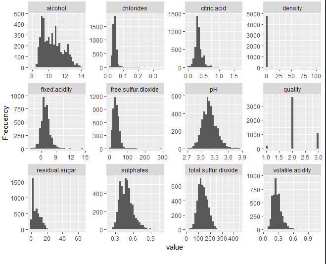
2.4 – DISTRIBUTION OF VARIABLES
Then, each of the available variables will be observed, studying if it exists, a priori, some anomalous or extreme data in them.
At Annexed 8.3: Variable distribution analysis everything is explained in greater detail, analyzing whether there is normality or asymmetry in the data, in addition to the Kurtosis coefficient.
A priori, anomalous data is not observed. As the only detail, in the density graph it can be seen that all the observations take values around 1.
These are some of the density values of some wines.
- Dry white wine: 0,9880-0,9930 g/mL.
- Dry red wine: 0,9910-0,9950 g/mL.
- Sparkling wine: 0,9890-1,0080 g/mL.
- Liquor wine (moscatel): 1,0500-1,0700 g/mL.
Thus, it's a normal value.
2.5 SCALING AND CENTERING DATA
After carrying out a small exploratory analysis of the data in this file, it is already passed to the part of the preprocessing, important part before carrying out the appropriate analyzes.
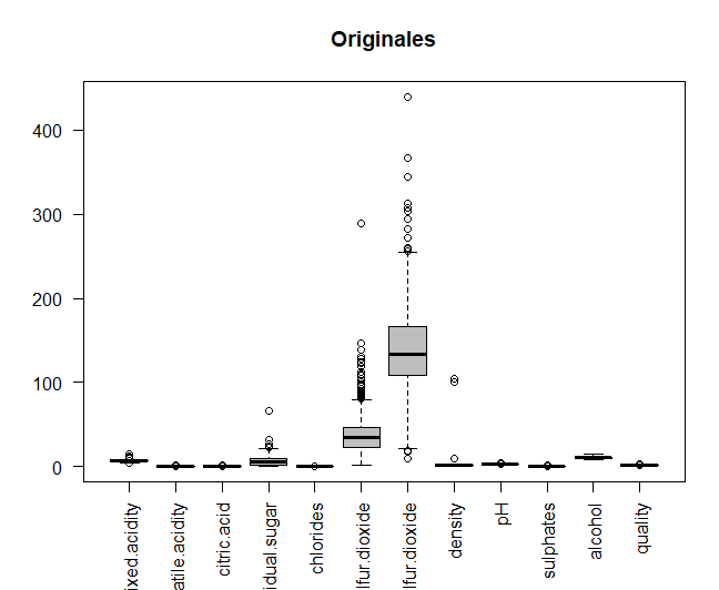
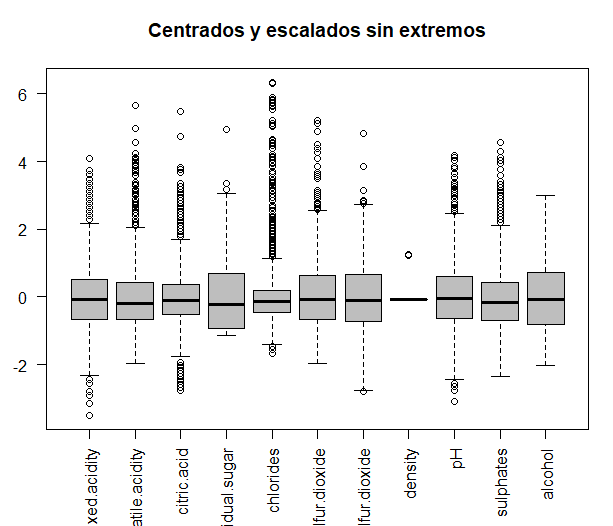
The original data will be compared with the data once centered and scaled, in order to see if the variables are measured at different magnitudes. Data is centered and scaled.
Then, the two graphs that make the comparison are printed in the same window, using the torque function. It can be seen how some of the variables are measured at different magnitudes, for example, the two types of sulfur. Thus, for further analysis, centered and scaled data will be used.

3. ANALYSIS 1 – PRINCIPAL COMPONENT ANALYSIS (PCA)
Once the exploratory analysis has been carried out and the data has been centered and scaled, you can go to the first of the three analyzes that will be carried out in this project of the subject. The first of them, as the title indicates, is the principal component analysis. The usefulness of this method is twofold:
- Optimally render in a small dimension space, observations of a p-dimensional general space. It is the first step to identify possible ‘latent’ or unobserved variables, that are generating the variability of the data.
- Allows to transform the original variables, generally correlated, in new uncorrelated variables, facilitating the interpretation of data.
3.1 OBJECTIVES
The objective when using this technique will be to obtain the variables that most influence the dimensions that explain the greatest variability. Using this method, it will be possible to obtain a more specific view of how the data being processed behaves. Apart, a small study will be carried out on some wines that have extreme data.
3.2 APPLICATION OF THE METHOD / NUMERICAL AND GRAPHIC RESULTS
SCREE-PLOT
It is already passed to the application of the method. All this is done through the PCA function already implemented in R. Data is not scaled because it has already been done previously.
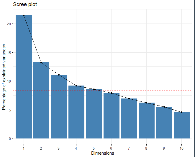
## eigenvalue variance.percent cumulative.variance.percent
## Dim.1 2.571633 21.434687 21.43469
## Dim.2 1.585109 13.211958 34.64665
## Dim.3 1.330253 11.087723 45.73437
## Dim.4 1.102265 9.187435 54.92180
## Dim.5 1.029659 8.582255 63.50406
The method is applied and it is observed how the ideal number of main components is 5. On one side, using the scree plot, the red line cuts into the fifth dimension. On the other hand, Another technique to choose the appropriate number of dimensions is to obtain those components which have an eigenvalue greater than 1. As well, Obtaining a table with said eigenvalue corresponding to each of the dimensions, it can be seen that, from the fifth component, the eigenvalue is greater than 1.
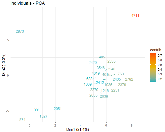
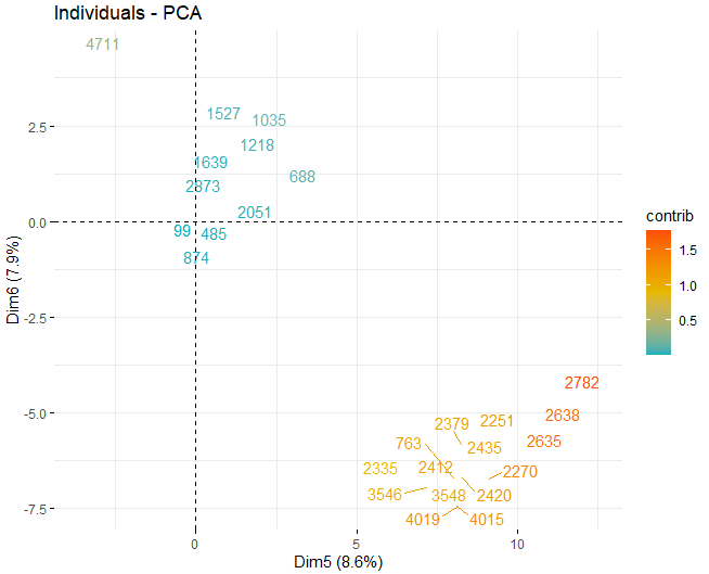
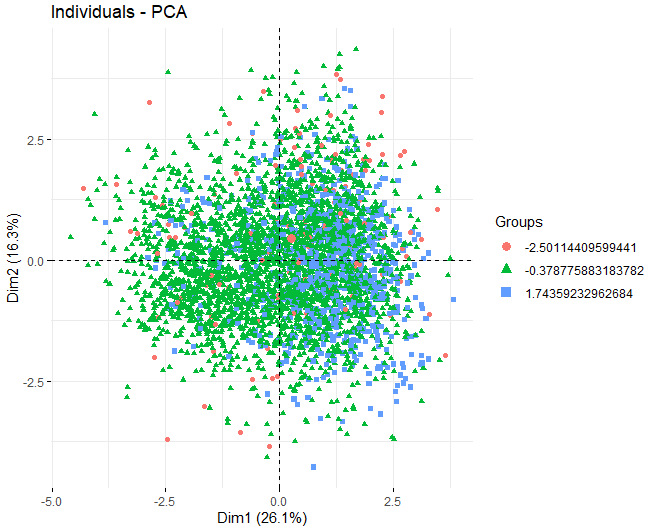
SCORE-PLOT
Then, a score plot is obtained with the scores of the wines in each of the dimensions that have been obtained previously. These wines are colored by their contribution in the components.
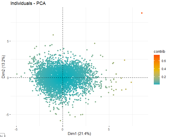
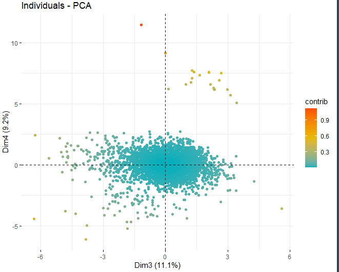
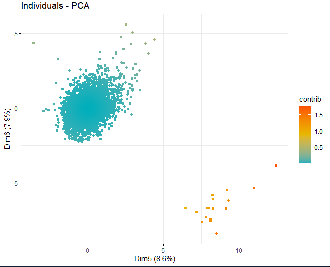
It can be seen how there are some anomalous values in the different components, apart from a few extreme observations that beat a score, in absolute value, greater than 5 and even from 10. In order to obtain more information on what these anomalous observations are, they go on to get the same score plots as before but, in this case, only with observations that exceed a score, in absolute value, of 5.
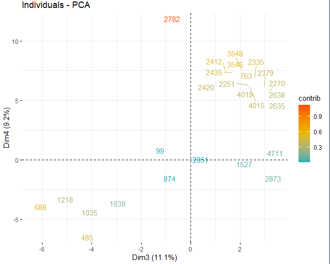
T2 HOTELLING
Some observations, specifically the wines 4711, 2782 The 2635, they have very extreme values that, if they are left in the database, may distort the conclusions of future analyzes. Specific, Any observations that exceed a limit of the 99% using Hotelling's T2.
Then, you can see some of the wines that exceed this limit.
It is observed that there are, specific, a total of 156 observations that exceed the 99%. 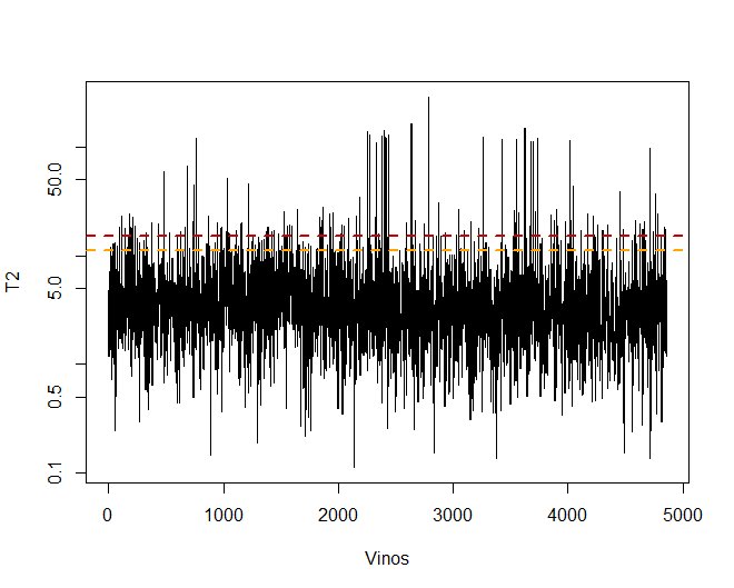
## [1] 156
Thus, for better analysis, these wines are eliminated.
## [1] 4702 12
Then, an auxiliary variable is created to store the quality variable in it, to be used in the following coloring analysis.
In this case, observing the ‘and’ axis of the boxplots, removing the previous values, extreme values no longer exist. 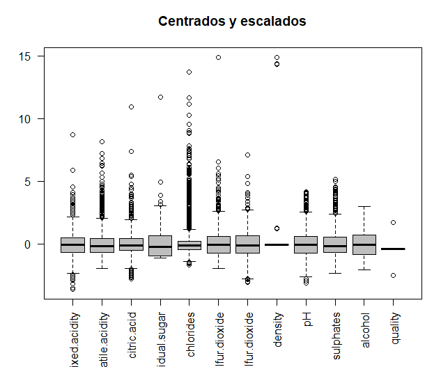
Now the PCA would have to be done again, with the new observations. In this case, following the same criteria as before (using the scree plot and the eigenvalues of each of the dimensions), are obtained 3 main components since they have an eigenvalue greater than 1.
## eigenvalue variance.percent cumulative.variance.percent
## Dim.1 2.3094622 26.079639 26.07964
## Dim.2 1.4442754 16.309503 42.38914
## Dim.3 1.0534806 11.896446 54.28559
## Dim.4 0.8526690 9.628779 63.91437
## Dim.5 0.8060166 9.101956 73.01632
LOADING-PLOT
Once the appropriate dimensions have been obtained, the loading plots of each of the dimensions that have been obtained previously are obtained: 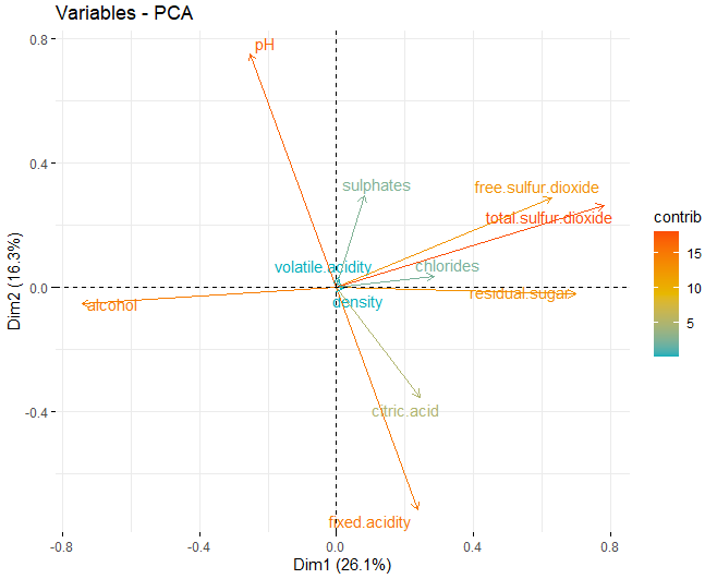
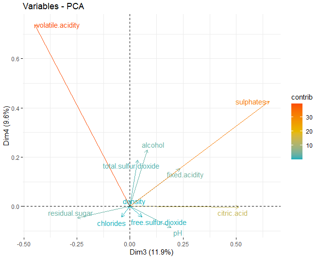
In this case it can be seen that, in the first dimension, the variables that most influence these dimensions are the physicochemical components of alcohol, residual sugar and the two types of sulfur, both free and total. On the other hand, in the second dimension, those that most influence are both pH and fixed acidity.
3.3 DISCUSSION OF RESULTS
In this first objective, it has been observed that it is necessary to carry out more than one PCA analysis due to the anomalous observations that may appear using the Hotelling T2.. If these results were ignored, probably the graphs of scores and loadings would not be interpreted in the same way and results would be obtained that would not be entirely real.
Aside from this, using this technique, it was possible to obtain a more detailed view of the database that is being processed, analyzing the variables that most influence the creation of dimensions. It has been observed that these are those of alcohol, residual sugar and the two types of sulfur, free sulfur and total.
4. ANALYSIS 2 – CLUSTERING
4.1 OBJECTIVES
The second analysis to be carried out in this project will be the analysis of conglomerates or cluster analysis. The objective when applying this technique in particular is to obtain which characteristics are the most important when evaluating the quality of a wine using hierarchical clustering techniques and partitioning algorithms.. In terms of this database, the objective is to obtain those chemical variables that influence the value that the response variable ends up taking, that is to say, la variable quality.
Finally, you will get a colored graph for quality, to study if really, the clusters that form these variables, are they well separated or not.
4.2 APPLICATION OF THE METHOD – NUMERICAL RESULTS
4.2.1 GROUPING THE DATA – HOPKINS STATISTIC
First of all, prior to the application of said method, you have to study if there is a grouping in the data being processed. This can be done using the Hopkins coefficient. It must be remembered that the closer this coefficient of 1, more grouping will exist in the data.
The hopkins function already implemented in R is used but, You have to be careful, because this function obtains the coefficient in a somewhat different way. Calculate the statistic backwards, that is to say, the real value of said coefficient is 1-H. Thus, in this case 1-0.08 = 0.92. Whereby, it can be said that there is a large grouping in the data.
## $H
## [1] 0.1029338
4.2.2 HCPC – HIERARCHICAL CLUSTERING ON PRINCIPAL COMPONENTS
The HCPC is an algorithm that groups similar individuals into clusters but with a peculiarity, is made to work with the results of a principal component method. This algorithm allows obtaining an optimal number of clusters using a technique based on inertia.. At Annexed 8.1: Bibliography A link is attached for more information about this.
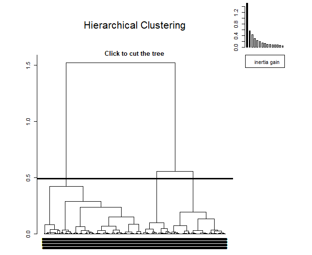
When applying it, can be seen as, at the top right, a small graph appears indicating the inertia in each of the dimensions. The method decides to take three clusters since, from the third component, inertia is maintained.
4.2.3 OBTAINING THE DISTANCE MATRIX
After presenting a first technique to obtain the optimal number of clusters, we go on to obtain the distance matrix, using the Euclidean distance since the objective is to find wines with similar characteristics to, later, study whether they are classified as good or bad.
4.2.4 WARD METHOD
First, Ward's method will be used. The first method has found the 3 as the optimal number of clusters, thus, k = 3 will be assigned.
## groups1
## 1 2 3
## 1743 2031 928
It can be observed that, using said method, the three groups formed seem to be well grouped, no seemingly anomalous data.
Then, Elbow and Silhouette methods will be used to validate the optimal number of clusters for Ward's method. 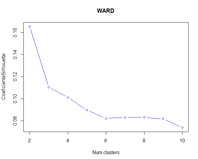
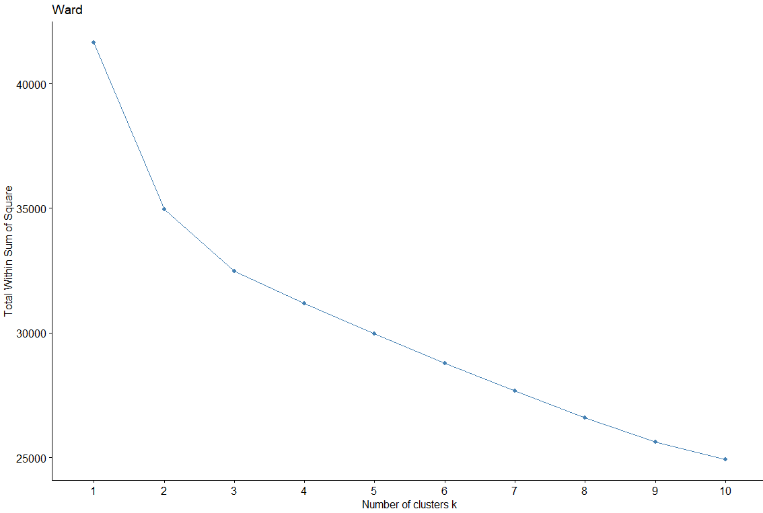
It is observed that, for both the Silhouette method and the elbow method (although it doesn't seem so clear), the optimal number of clusters would be 2 clusters. In this case, using two clusters, more than 1000 observations in one group relative to another.
## groups1b
## 1 2
## 1743 2959
4.2.5 K-MEANS
Next another method is studied, in this case the Kmeans or Kmedias method. Like it has been done with Ward's method, k = 3 will also be assigned in this case. A good grouping of the data is also observed using three clusters..
##
## 1 2 3
## 1683 1475 1544
The optimal clustering method is obtained using this method., also with Silhouette coefficient and elbow method. 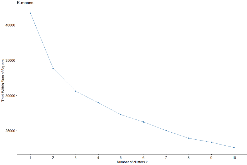
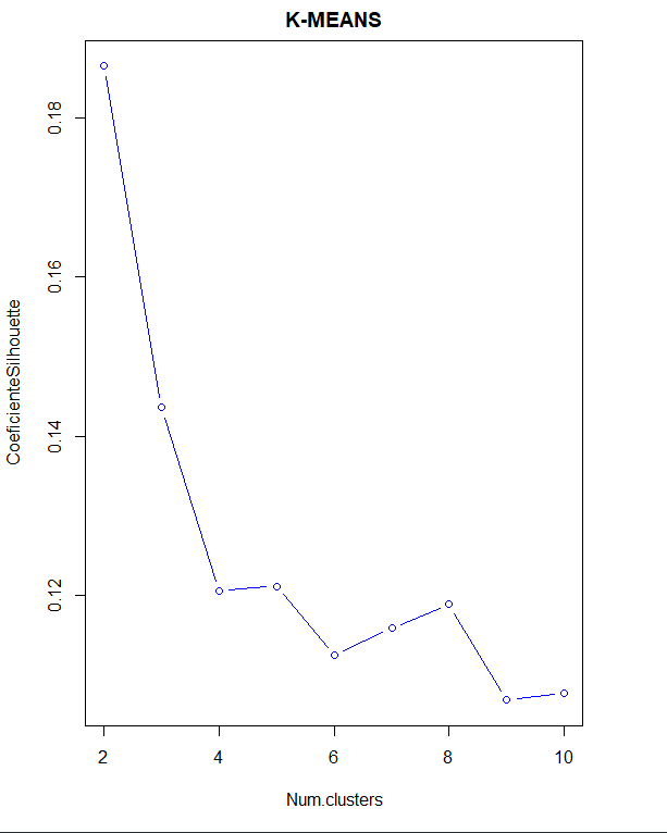
In this case, in the elbow method, you don't see such a defined elbow. However, studying the Silhouette coefficient, indicates that the number of clusters is 2 again.
4.3 OPTIMAL NUMBER OF CLUSTERS – VALIDATION OF THE RESULTS
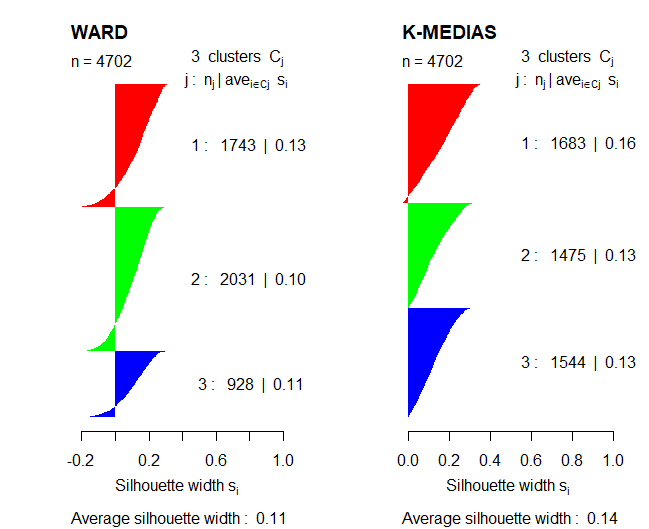
After studying some methods to obtain the optimal number of clusters, these methods will be compared using the Silhouette coefficient in order to validate the results.
Comparing the two representations, you can tell the partition method, the k-means algorithm, works better than Ward's hierarchical method because Silhouette's coefficient is higher in that case. Also, in the case of Ward's method, a few observations appear with negative values in the coefficient being used.
Thus, in the next section, the interpretation of the clustering results will be studied using the K-means method. Also, this algorithm will be used with 3 clusters since, previously, it has been observed that with that K value, groups were more balanced, no anomalous values.
4.4 GRAPHIC RESULTS
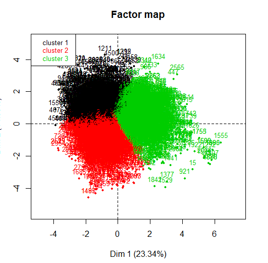
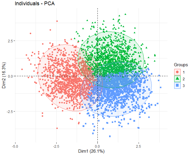
Having commented that the K-means method will be used, we proceed to obtain a PCA to see which variables contribute the most in the formation of the clusters. In this case, It can be observed that, using the k-means algorithm with 3 clusters, the 3 groups separate very well, they are balanced.
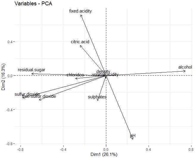
It can be observed that, in the first two dimensions, the variables that most influence the creation of clusters are residual sugar, the alcohol, and the two types of sulfur, both total sulfur and free sulfur.
Finally, we go on to show a graph where each of the wines is represented to see if the quality variable influences the creation of the clusters. You can see that the clusters are not well separated, most points overlap with others.
4.5 DISCUSSION OF RESULTS
Through this technique it has been observed that the quality variable does not influence the creation of the clusters. This could be due to different factors that have not been taken into account in the analysis from the beginning.. Clusters may be formed according to other variables such as, the appellation of origin, the type of grape that is being used to make these wines, etc.
5 ANALYSIS 3 – PARTIAL LEAST SQUARES – DISCRIMINANT ANALYSIS (PLS-DA)
The PLS technique is a mix between multiple regression and PCA. Keep in mind that if there is multicollinearity, the regression may not be performed correctly and the desired results may not appear. However, the PLS previously uses the PCA to observe which variables are the most influential in the creation of the variables that are being studied and each of the components is orthogonal to the next one that most influences and so on. For that reason, thanks to the fact that the components are linearly independent from each other, the regression can be carried out without any problem.
One of the PLS variants is the PLS-DA, which is the one to be used in this project, which includes the discriminant analysis technique. The difference, with respect to the prior art, is that the response variable is categorical. From this categorical variable, as many ‘Dummy’ variables will be created as there are different values that response variable can take..
5.1 OBJECTIVES
The objective when using this technique is twofold. On one side, study possible anomalous observations (then, it will be explained how to treat them). On the other hand, evaluate the predictive capacity of a PLS-DA model with the wine quality variable.
In the first technique that has been used, the of the PCA, it has been observed that, using Hotelling's T2, some observations appeared that exceeded the 99%, considering anomalous and extreme observations those that were farthest from that cut. A similar procedure will be carried out in the PLS. Firstly, a first PLS model will be made and, using the Hotelling T2 technique, possible anomalous or extreme observations will be studied.
Any observations that exceed the limit of the 99% using Hotelling's T2 and then a new PLS model will be created again, in order to obtain a more reliable model than another with anomalous cases that may alter its characteristics.
5.2 APPLICATION OF THE METHOD
It goes on to the application of the model. First you have to transform the response variable to factor since, although it is qualitative, the program does not detect it that way since it takes numerical values.
Once applied, you can see how the model gets 3 as ideal number of components.
## PLS-DA
## 4858 samples x 11 variables and 1 response
## standard scaling of predictors and response(s)
## R2X(cum) R2Y(cum) Q2(cum) RMSEE for ort pR2Y pQ2
## Total 0.405 0.116 0.113 0.337 3 0 0.05 0.05
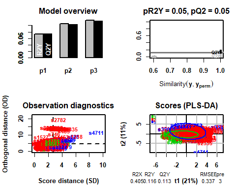
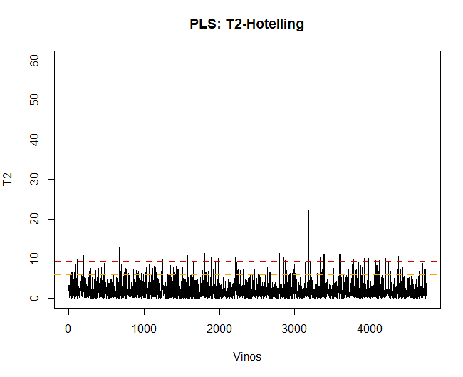
5.2.1 T2-HOTELLING
The first thing to do, once the model is applied, is the validation of the data, observe if there are abnormal or extreme observations that may influence the results. For it, a graph of Hotelling's T2 will be made and thus be able to detect them.
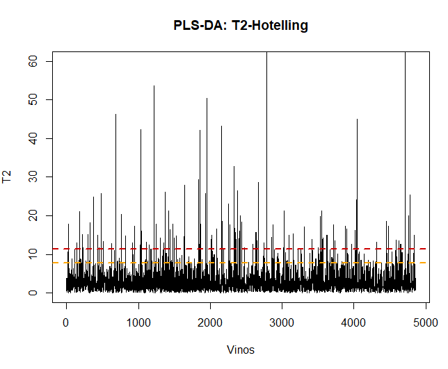
Using this technique, you can see there are some 100 anomalous observations. Such data will be removed and the PLS-DA model will be reapplied.
## [1] 109
5.3 APPLICATION OF THE METHOD WITHOUT ANOMAL DATA
In this case you can see that, removing the previous observations, the model chooses in this case 2
## PLS-DA
## 4749 samples x 11 variables and 1 response
## standard scaling of predictors and response(s)
## R2X(cum) R2Y(cum) Q2(cum) RMSEE for ort pR2Y pQ2
## Total 0.31 0.104 0.101 0.337 2 0 0.05 0.05
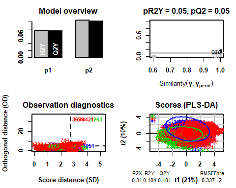
5.3.1 T2-HOTELLING
If the Hotelling T2 graph is now displayed, There are no longer anomalous data that can influence the model.
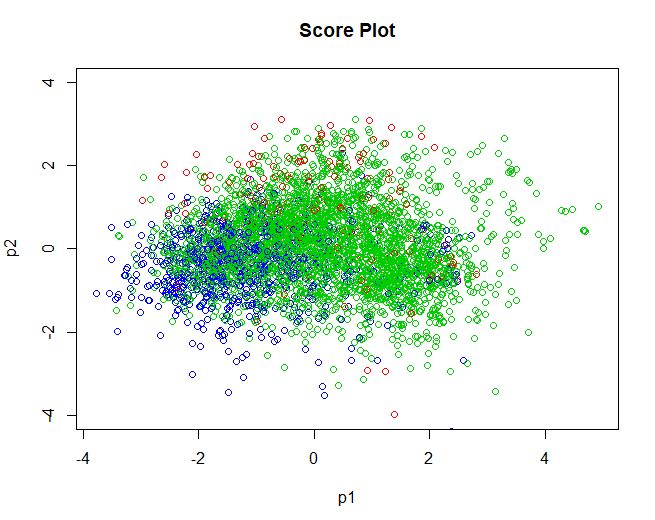
5.3.2 SCORE-PLOT
Once the data is validated, we go on to obtain the score graph, relating to individuals. Very similar results are obtained to those obtained using the k-means algorithm used in the Analysis 2. Groups are not clearly separated, most overlap with each other. As mentioned in the previous analysis, this could be because the groups are not separated by quality, but by other variables that in this analysis have not been arranged such as the designation of origin of the wine, the type of grape used to make it, etc.
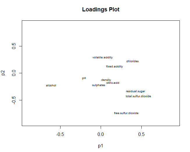
5.3.3 LOADING-PLOT
On the other hand, we pass to graph the loadings graph, referring to variables. In this case, the results are very similar to those obtained in the principal component analysis.. Total sulfur, free sulfur and alcohol, have a high contribution in both dimensions. However, using PLS-DA it is obtained that the pH does not contribute in any of the two components (in PCA had a great contribution in the second component)
5.4 PLS-DA MODEL PREDICTION
In this fourth section, the prediction of the model used in this third analysis will be made.. By having some 5000 observations, we go on to create a training set and a test set.
## PLS-DA
## 3800 samples x 11 variables and 1 response
## standard scaling of predictors and response(s)
## R2X(cum) R2Y(cum) Q2(cum) RMSEE for ort pR2Y pQ2
## Total 0.307 0.0982 0.0937 0.338 2 0 0.05 0.05
5.4.1 TRAINING SET
Using the training data, it can be seen that the model has an accuracy of 76,55%, which is a very acceptable value. However, look closely at the observations you predict for each of the groups. This precision value is high because it classifies almost all the wines in the group well. 2 ("Good" with a rating between 5 and 7). Classifies 2801 wines in the group 2, and the 43 remaining to group 3.
However, of the first group has not classified any of these well (120 in the group 2 and 1 in the group 3). Finally, in the group 3 has classified 108 observations belonging to that group and 727 for the group 2.
Thus, it can be said that the model predicts the wines of the second group very well. Due, the precision value is high.
## Confusion Matrix and Statistics
##
## mypred
## 1 2 3
## 1 0 120 1
## 2 0 2801 43
## 3 0 727 108
##
## Overall Statistics
##
## Accuracy : 0.7655
## 95% CI : (0.7517, 0.7789)
## No Information Rate : 0.96
## P-Value [Acc > NIR] : 1
5.4.2 TEST SET
Finally, to validate the model, the same will be done before but, in this case, with observations the model has not previously seen (test set)
A trend similar to that of the training set can be observed. The model has an accuracy of 76,92%, value very similar to that obtained in the other set. However, as previously discussed, the model classifies only the wines of the group very well 2 but the other two groups don't distinguish them well.
## Confusion Matrix and Statistics
##
## mypred
## 1 2 3
## 1 0 30 0
## 2 0 692 19
## 3 0 170 38
##
## Overall Statistics
##
## Accuracy : 0.7692
## 95% CI : (0.7411, 0.7957)
## No Information Rate : 0.9399
## P-Value [Acc > NIR] : 1
6 CONCLUSIONS
6.1 COMPARISON OF THE METHODS USED
Finally, in this project three methods have been used for the three corresponding analyzes: Principal component analysis, Clustering y Partial Least Squares – Discriminant Analysis (PLS-DA).
The first method, the PCA, has served to obtain a preprocessing of the data and in this way, to be able to study the database a little more thoroughly, Analyzing the variables that have the most contribution in the main dimensions that have been obtained. Similar results could be found between the PCA and the PLS-DA, this is, analyzing the loading-plot of both techniques, the same variables that contributed more in the two techniques have been obtained, excepting some exceptions.
On the other hand, the PCA, thanks to the cleaning that has been done in the database, has served for the second analysis, clustering, since it has allowed obtaining the clusters in a more balanced way, no abnormal groups with few observations.
Finally, the PLS-DA method, in addition to what has been commented previously about the similar results obtained with the PCA, has been used to evaluate the predictive capacity of the model. A good first model has been obtained but it should be improved in the future, because groups with lower observations were not predicted correctly.
6.2 DISCUSSION ON NON-APPLIED METHODS
Three methods have not been used in this project: Factorial Analysis of Correspondences (AFC), Association Rules and Discriminant Analysis. The first two techniques were not used because the database that was used for this work did not have qualitative variables. (only the response variable, wine quality). The fact of transforming all the variables could have caused a significant loss of information.
On the other hand, Discriminant analysis was also a good option to obtain the variables that most influenced when discriminating between the different groups in which the wines were classified and subsequently, classify new observations. PCA and clustering had already been applied and, because the completion of the PLS was mandatory, this method could not be studied.
Finally, The PLS-DA technique has been used within the PLS because the response variable was qualitative. In this way, said variable has been used as Y and the other physical-chemical variables as X.
7. OTHER THEMES
7.1 COMMENTS ON READ ARTICLES
It has been possible to study that the different groups do not separate well due to the quality. Thus, seen this, it was decided to do a little research about what this group might look like. Through some news and articles it has been possible to know that the quality of the wine is not a linear combination of the physical-chemical variables that were available. Thus, the valuation of a wine is not linear, has buggy trends. These errors are influenced by the criteria of each judge.
Thus, la variable ‘quality’, in the case of being obtained from evaluations of expert judges, It has certain inaccuracies that are due to the tastes of each of these.
8. ANNEXED
8.1 BIBLIOGRAPHY
- Wine characteristics manual
- How do I know if I am enjoying a quality wine??
- HCPC
- Practical Guide To Principal Component Methods in R (Kassambara)
- FactoMineR
- MULTIVARIANT DATA ANALYSIS – Daniel Peña
- THE ELEMENTS OF STATISTICAL LEARNING
8.2 DISTRIBUTION ANALYSIS OF VARIABLES
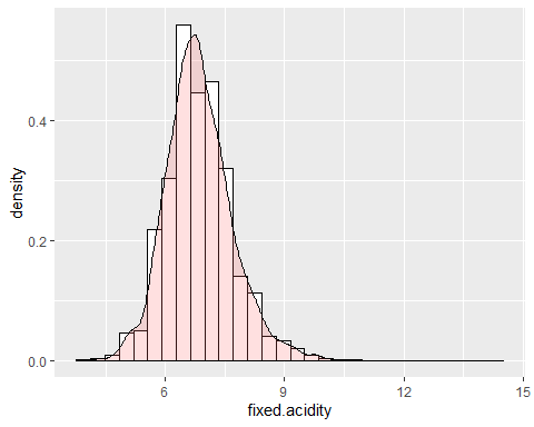
FIXED ACIDITY HISTOGRAM
The first of the variables is the fixed acidity. This variable has an asymmetry of 0.647 but a kurtosis of 5.16. This indicates that said variable does not follow a normal distribution. Besides, an extreme data is observed which takes the value of 14,2.
HISTOGRAM VOLATILE ACIDITY
Volatile acidity has a shape similar to the previous variable. This variable has an asymmetry of 1,576 and a kurtosis of 8,08 which also indicates that it does not follow a normal distribution.
It is observed that the two previous variables have long and positive tails and, because of this, the mean is much higher than it should be. 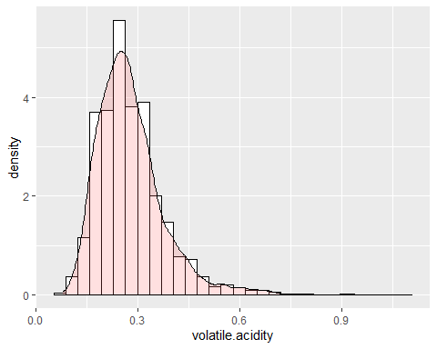
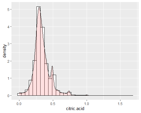
CITRUS ACID HISTOGRAM
In the acid some atypical data can be observed such as 1,66 g / dm ^ 3 that marks the maximum of the variable. Apart of this, an asymmetry of 1,28 and a kurtosis of 9,16. Thus, nor does it follow a normal distribution.
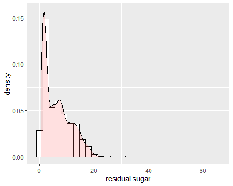
RESIDUAL SUGAR HISTOGRAM
Residual sugar has a positive bias. It is observed that it has an asymmetry of 1,07 and a kurtosis of 6,46, that is to say, does not follow a normal distribution. A very high peak is observed.
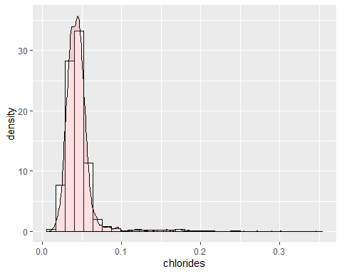
CHLORINE HISTOGRAM
Chlorine has several extreme data with a kurtosis coefficient of 40,52. It also has a positive asymmetry with a coefficient of 5,02. Therefore, said variable is not distributed according to the Gaussian bell..
TOTAL AND FREE SULFUR DIOXIDE HISTOGRAMS
Distributions for sulfur dioxide, both free and total, are symmetric because they have skew coefficients of 1,40 and 0,39 respectively. In both cases there are extreme data (short of 14,45 and 3,57). They do not follow a normal distribution. 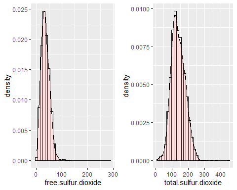
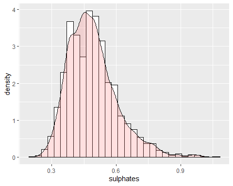
SULPHATE HISTOGRAM
Sulfate has a positive skewness with a coefficient of 0.9768. Since it has a kurtosis coefficient higher than 2, anomalous data exists and, so, does not follow a bella de Gauss.
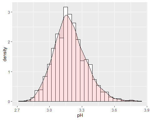
PH HISTOGRAM
The pH of the wine is around 3,15 with some anomalous data because the kurtosis coefficient is higher than 2.