Pollution and traffic 2020 (lockdown) and 2017

Pollution and traffic evolution 2020 (lockdown) compared to 2017 on the same dates

Introduction:

Pollution and traffic 2020 (lockdown) compared to 2017

A study of the evolution of traffic and pollution in Valencia with and without the Coronavirus will be carried out on the same dates, differing in the year only.

The following traffic data is available:

Traffic data according to different sections of Valencia from 02/05/2017 until the 16/05/2017 (Period without confinement)
Traffic data according to different sections of Valencia from 28/04/2020 until the 12/05/2020 (Period with confinement)

As you can see, the dates don't seem to match, but they do match, since they both start on Tuesday and end 2 weeks later. As can be seen below, both data include non-working and non-working days..

1. Analysis and evolution of traffic and pollution

Pollution and traffic 2020 (lockdown) compared to 2017

-1.1 Average traffic during 15 days.

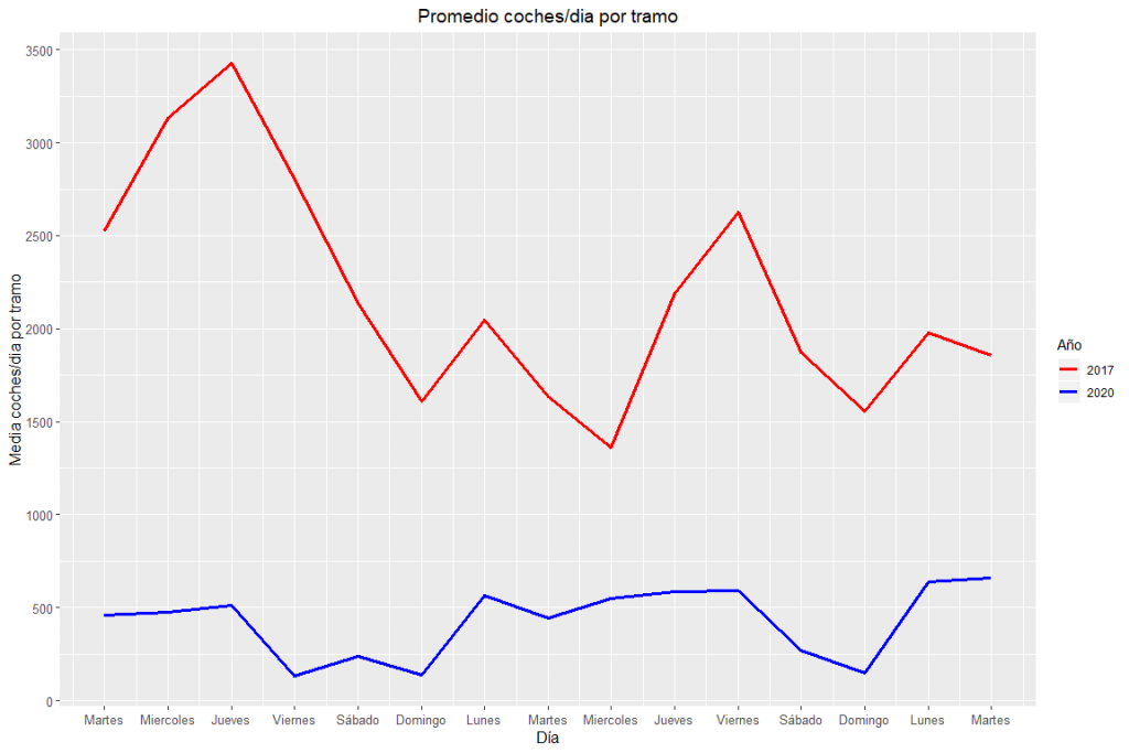
First of all, a little analysis will be done, roughly, to observe how traffic evolves in the 15 days that have been selected, comparing 2017 with 2020. In this case, a line graph will be shown in which the X axis represents the temporal axis (days) and, the y axis, the average number of cars passing a section in Valencia per day.

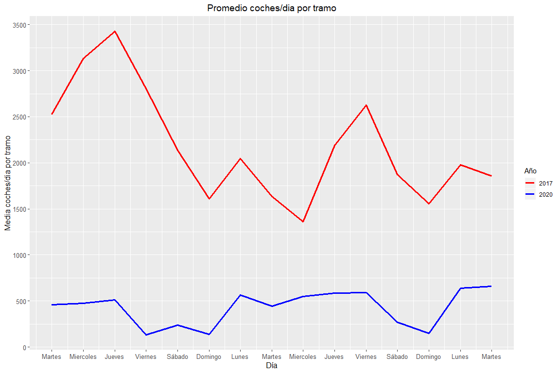
Evolution of general traffic in Valencia in 2017 and 2020.

As expected, traffic volume during confinement decreases a great deal over the same period in 2017 without confinement.

Then, the trend of pollutant levels in the two periods will be analyzed. Thus, it will be possible to see in a very precarious way some relationship between traffic and the levels of pollutants if they exist.

Pollution and traffic 2020 (lockdown) compared to 2017

-1.2 Pollution levels of pollutants:

Clarification: all measurements come from the Pista de Silla contamination station.

Pollution and traffic 2020 (lockdown) compared to 2017

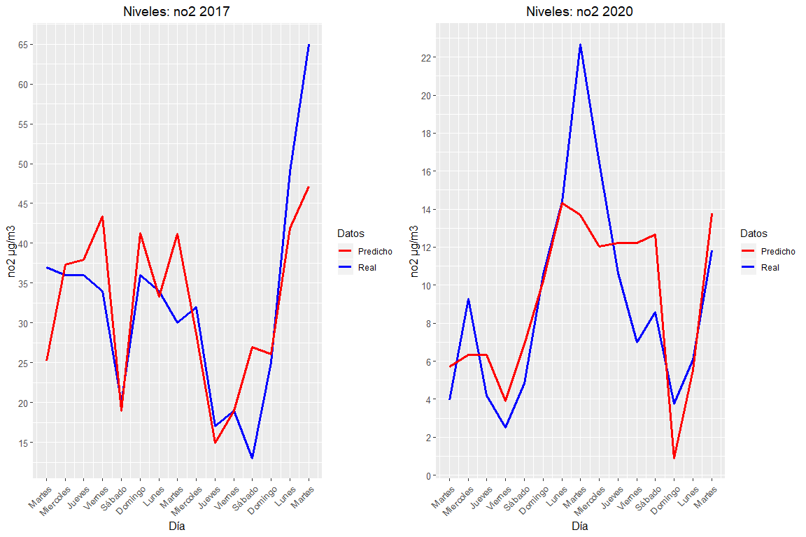
-1.2.1 NO2 (Nitrogen dioxide)

NO2 is a polluting agent that is produced when Oxygen and Nitrogen meet at high temperatures. This process can occur in engines of internal combustion, lightning storms, acid rains, coal power plants, etc ... This pollutant can cause irritation to the lungs and, as a result of this, decrease resistance to respiratory infections.

The higher the NO2 levels the worse for human health.

Then, NO2 values will be displayed during the time period described above, so much of 2017 like 2020:

“The values of No. 2 in 2017 They are a 253% greater than 2020 values”

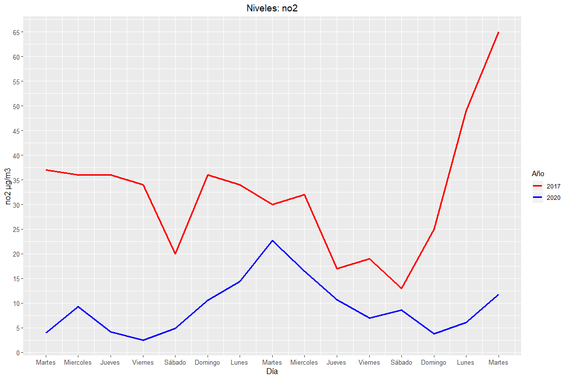
Evolution of NO2 levels in Valencia in 2017 and 2020.

As can be seen in the graph above, the average NO2 contamination levels in 2017 son 3.5 NO2 values in 2020. Follows a similar trend in the two years, However, in 2017 there are more extreme values. Specific, on the last Tuesday, a more pronounced peak is observed.

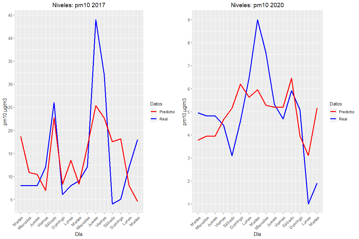
-1.2.2 PM10 (Suspended particles less than or equal to 10 microns per cubic meter)

PM10 is a contamination meter, Specifically, it determines the number of particles in suspension with a size less than or equal to 10 microns found in the environment. They are not a big health problem as long as they are larger than 2.5 microns since the body can expel them through the mucus or, do not reach the respiratory tree. These particles are created, mainly in combustion processes.

The higher the PM10 levels, worse for human health.

Then, PM10 values will be displayed for the time period described above, so much of 2017 like 2020:

“Pm10 values in 2017 They are a 188% greater than 2020 values”

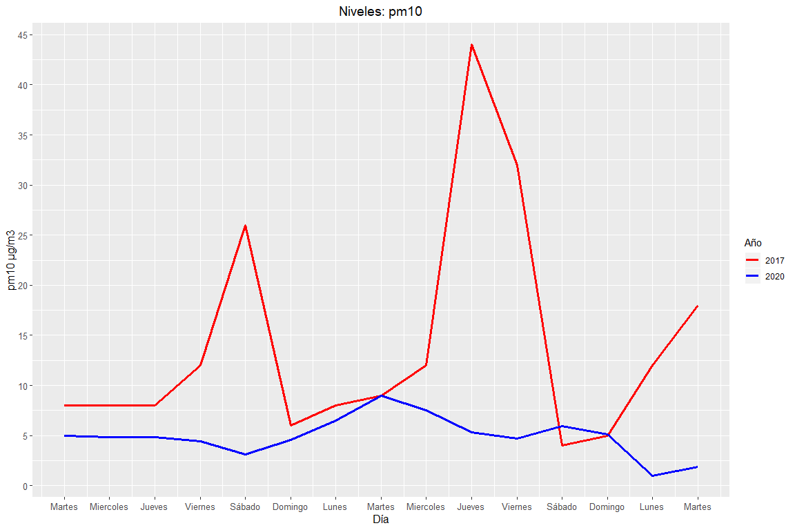
Evolution of PM10 levels in Valencia in 2017 and 2020.

As can be seen in the graph above, mean PM10 levels in 2017 son 2.8 PM10 values in 2020. In this case, PM10 trends do not vary much, you can see how, in 2020, PM10 levels are almost unchanged and are kept at fair values. However, PM10 values in 2017 they are higher on average and there are also certain extreme values on the first Saturday, the second Thursday and the second Friday which are very high.

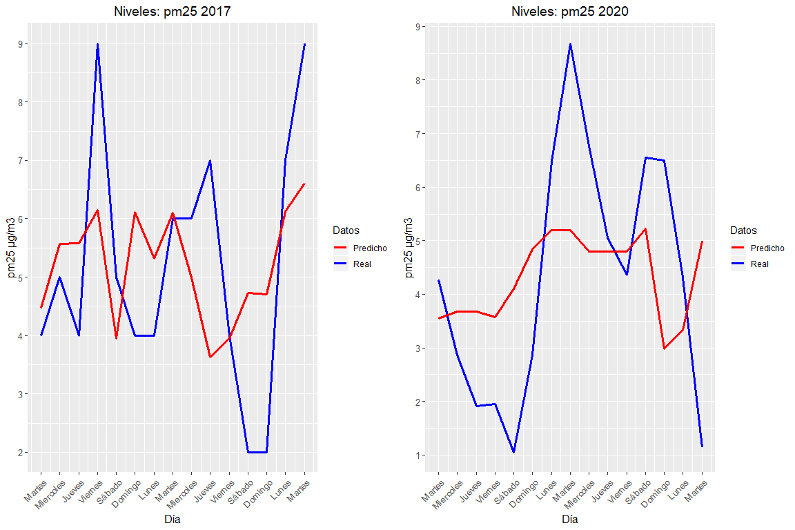
-1.2.3 PM2.5 (Suspended particles less than or equal to 2.5 microns per cubic meter)

PM2.5 is a contamination meter, Specifically, it determines the number of particles in suspension with a size less than or equal to 2.5 microns found in the environment. These pose a great problem since the body cannot expel them easily and they reach the respiratory tree thus causing respiratory diseases., allergies, etc ... These particles are created, mainly, in combustion processes.

The higher the PM2.5 levels, worse for human health.

Then, PM2.5 values will be displayed during the time period described above, so much of 2017 like 2020:

“The pm25 values in 2017 They are a 20% greater than 2020 values”

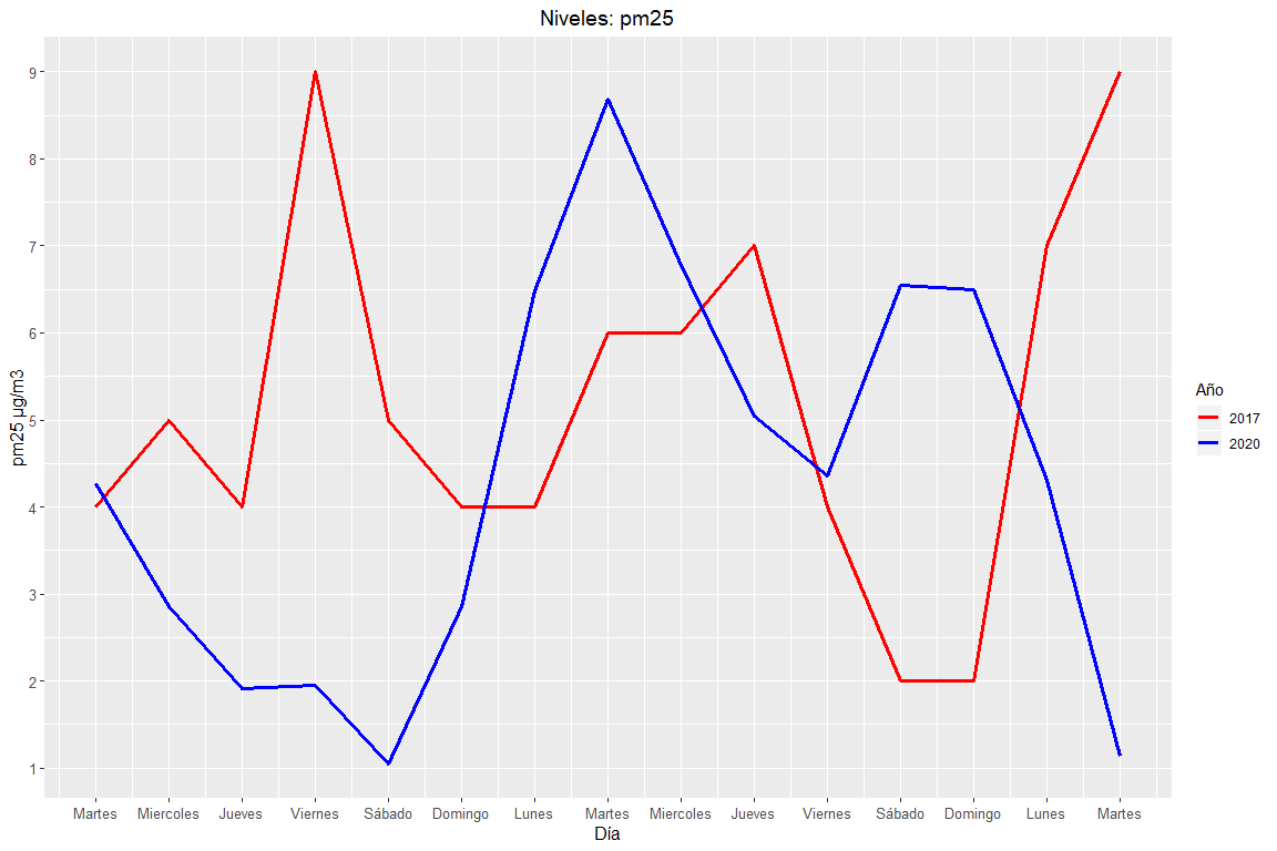
Evolution of PM2.5 levels in Valencia in 2017 and 2020.

As can be seen in the graph above, the average PM2.5 levels in 2017 son 1.2 PM10 values in 2020. In this case, PM2.5 trends vary quite a bit, you can see how in 2020, PM2.5 levels stay low during the week and rise once the weekend begins. It can be seen how PM2.5 levels undergo a number of variations in both years. There are also no big differences in both years, they are quite similar.

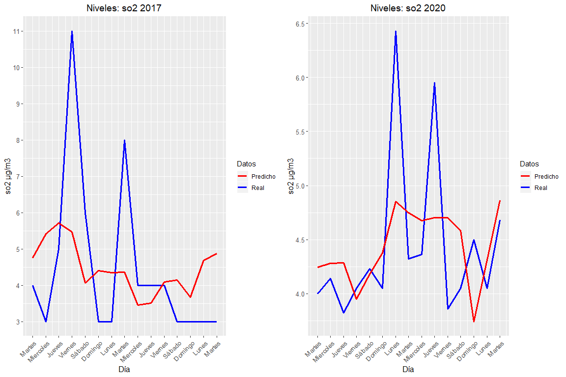
-1.2.4 SO2 (Sulfur dioxide)

SO2 is a colorless and irritating gas polluting the air. This is produced by the combustion of poorly refined fuels, in which there is a high presence of sulfur. So, Today's vehicles that use refined fuels are not causing a significant effect on SO2 levels.

The higher the SO2 levels, worse for human health.

Then, SO2 values will be displayed during the time period described above, so much of 2017 like 2020:

“So2 values in 2017 They are a 1% greater than 2020 values”

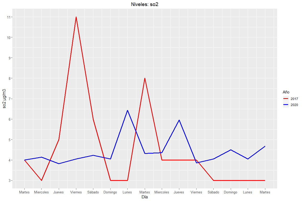
Evolution of SO2 levels in Valencia in 2017 and 2020.

In this case it is seen that the year 2017 has higher SO2 peaks, but they both have the same average approx. So, there are no big differences between the SO2 levels of 2017 and 2020.

-1.2.5 O3 (Ozone)

Ozone is a colorless gas that is present in the air and can be harmful if its concentration is high and is maintained over time.. Causes respiratory diseases.

The higher the levels of O3 the worse for human health. But it must be emphasized that low concentrations of this gas do not produce any effect on health.

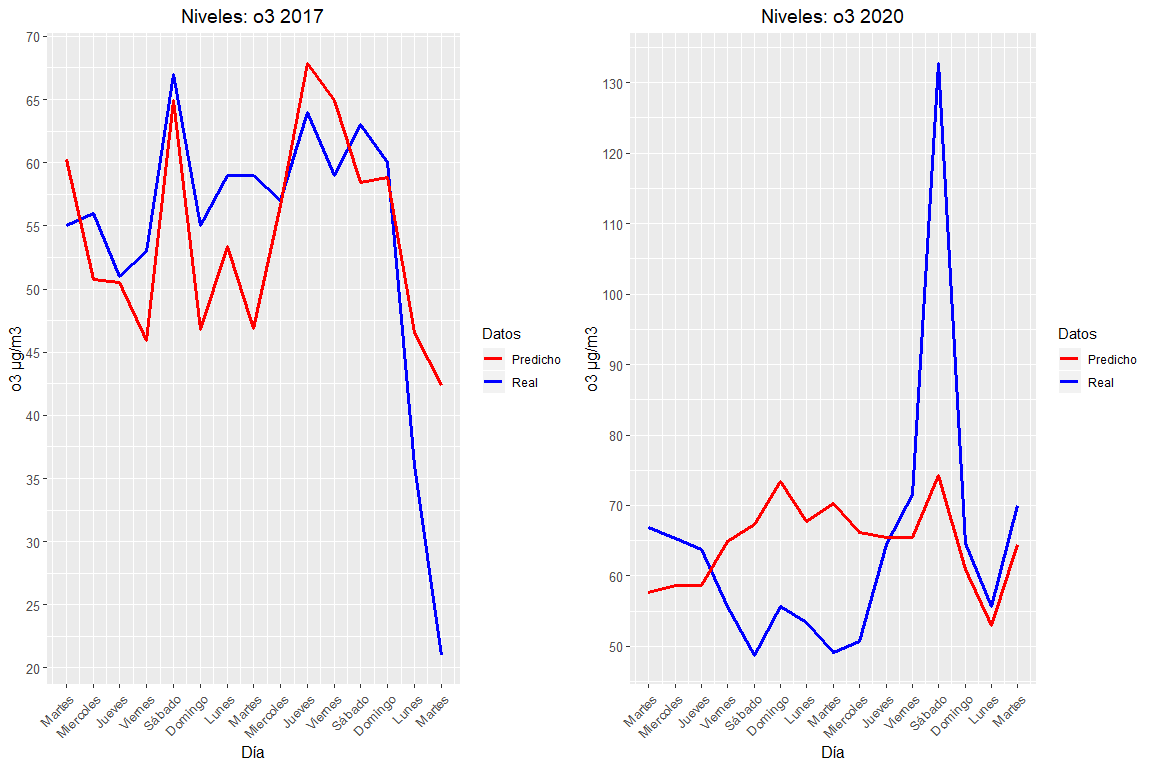
Then, O3 values will be displayed for the time period described above, so much of 2017 like 2020:

“The o3 values in 2017 They are a 16% less than 2020 values”

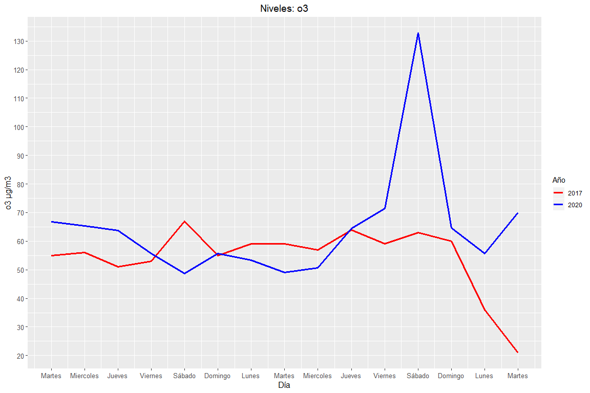
Evolution of O3 levels in Valencia in 2017 and 2020.

In this case it is seen that 2020 has higher peaks of O3 levels, in addition to that the average levels of O3 in 2020 are greater than the average levels in 2017. This may be because, lately the use of 03 to disinfect objects,specific, to remove copies of Coronavirus present on objects.

2 Traffic ratio – contamination

Pollution and traffic 2020 (lockdown) compared to 2017

Doing a little research on what factors are causing pollution in the city, it is obtained that the majority of the sources place internal combustion vehicles as the main causes of pollution. Too, most sources affect the importance of wind in reducing pollution levels since, at higher wind speed, the air contaminated it is renewed more easily, and the polluting particles disperse more, thus reducing its harmful effect. For all this, it has been decided to study the relationship between traffic and pollution taking into account the wind.

First, a correlation graph will be made to see if there are linear relationships

-2.1 Daily traffic correlation, wind and level of pollutants of the year 2020

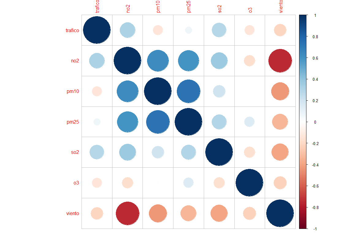
Correlation graph between traffic, wind and pollutants

Pollution and traffic 2020 (lockdown) compared to 2017

As you can see, traffic has a positive correlation with pollutants no2 and so2, which could indicate that the greater the number of internal combustion vehicles, the higher the levels of pollutants no2 and so2. You can also see that there is very little correlation between traffic, pm10, pm25 and o3 so it could indicate that these pollutants are not related to traffic at all.

Also noteworthy is the role of wind with all pollutants. In this case, all correlations are negative, which could indicate that, the higher the wind, lower are the levels of contamination.

By last, it should be noted that the PM10 and PM2.5 meters have a large positive correlation, which in this case is obvious since both measure particles in suspension with common characteristics.

2.2 Simple regression model

In order to determine if there is any relationship between pollution and traffic variables, we will try to fit a regression model to the data., in which the dependent variable will be a polluting agent and the independent variables will be traffic and wind.

2.2.1 Input data

In this case, Pollutant levels have been taken at the Pista de Silla contamination station and the traffic values belong to the average of the two sections closest to this station.. Once the data is crossed, the following dataset is obtained (the 6 first rows only)

head(generatedata(“2020”))

## traffic no2 pm10 pm25 so2 o3 wind
## 1 358 3.95 4.95 4.27 4.00 66.86 3.3
## 2 354 9.27 4.82 2.86 4.14 65.32 3.1
## 3 356 4.20 4.82 1.91 3.82 63.82 3.1
## 4 87 2.50 4.41 1.95 4.05 55.68 3.3
## 5 136 4.83 3.09 1.05 4.23 48.73 2.5
## 6 92 10.58 4.59 2.86 4.05 55.68 1.4

The data is per day, so, each row of the dataset corresponds to one day. Example: Row one indicates that that day has passed 358 average cars for the two sections near the Silla Track Pollution station, that the average wind speed has been 3.3 m/s (11.88 km / h) and later, the columns of the pollutants, indicate the mean values of these contaminants in micrograms / cubic meter.

2.2.2 Model

The model will try to predict the levels of pollutants through wind and traffic:

y = x0 + x1 + x2

Pollutant Agent Level = intercept + cars / day + medium wind

2.2.2.1 NO2

“Regression model of 2017 for no2”
## lm(formula = pollutant ~ wind + traffic)
## Coefficients:
## Estimate Std. Error t value Pr(>|t|)
## (Intercept) 50.141935 9.872786 5.079 0.000271 ***
## wind -10.926847 2.604092 -4.196 0.001241 **
## traffic 0.001598 0.003441 0.464 0.650667
## Signif. codes: 0 ‘***’ 0.001 ‘**’ 0.01 ‘*’ 0.05 ‘.’ 0.1 ‘ ‘ 1

## Residual standard error: 8.994 on 12 degrees of freedom
## Multiple R-squared: 0.5973, Adjusted R-squared: 0.5302
## F-statistic: 8.899 on 2 and 12 DF, p-value: 0.004265

“Regression model of 2020 for no2”
## lm(formula = pollutant ~ wind + traffic)
## Coefficients:
## Estimate Std. Error t value Pr(>|t|)
## (Intercept) 14.275114 3.362760 4.245 0.00114 **
## wind -3.315617 0.896657 -3.698 0.00305 **
## traffic 0.006595 0.007389 0.893 0.38967
## Signif. codes: 0 ‘***’ 0.001 ‘**’ 0.01 ‘*’ 0.05 ‘.’ 0.1 ‘ ‘ 1

## Residual standard error: 3.891 on 12 degrees of freedom
## Multiple R-squared: 0.5803, Adjusted R-squared: 0.5103
## F-statistic: 8.295 on 2 and 12 DF, p-value: 0.005468

Thanks to the graphs and the statistical summary it is possible to determine that both models, both the of 2020 such as 2017 are significant since their P-values are less than 0.05. Also, it can also be seen how in both models the only significant variable is the wind. This indicates that the only variable that is related to NO2 levels is the wind. Also, due to the negative value of your estimator x1 = -3.31, it can be inferred that, at higher average wind speed, lower will be the levels of this pollutant.

2.2.2.2 PM10

“Regression model of 2017 for pm10”
## lm(formula = pollutant ~ wind + traffic)
## Coefficients:
## Estimate Std. Error t value Pr(>|t|)
## (Intercept) 2.583639 11.015327 0.235 0.8185
## wind 7.063502 2.905454 2.431 0.0317 *
## traffic -0.001051 0.003839 -0.274 0.7889
## —
## Signif. codes: 0 ‘***’ 0.001 ‘**’ 0.01 ‘*’ 0.05 ‘.’ 0.1 ‘ ‘ 1

## Residual standard error: 10.03 on 12 degrees of freedom
## Multiple R-squared: 0.3323, Adjusted R-squared: 0.221
## F-statistic: 2.986 on 2 and 12 DF, p-value: 0.08861

“Regression model of 2020 for pm10”
## lm(formula = pollutant ~ wind + traffic)
## Coefficients:
## Estimate Std. Error t value Pr(>|t|)
## (Intercept) 7.637333 1.614814 4.730 0.000489 ***
## wind -0.813163 0.430579 -1.889 0.083361 .
## traffic -0.003312 0.003548 -0.933 0.369072
## —
## Signif. codes: 0 ‘***’ 0.001 ‘**’ 0.01 ‘*’ 0.05 ‘.’ 0.1 ‘ ‘ 1

## Residual standard error: 1.868 on 12 degrees of freedom
## Multiple R-squared: 0.2437, Adjusted R-squared: 0.1177
## F-statistic: 1.934 on 2 and 12 DF, p-value: 0.1871

2.2.2.3 PM2.5

“Regression model of 2017 for pm25”
## lm(formula = pollutant ~ wind + traffic)
## Coefficients:
## Estimate Std. Error t value Pr(>|t|)
## (Intercept) 7.134e+00 2.287e+00 3.120 0.00886 **
## wind -9.983e-01 6.032e-01 -1.655 0.12384
## traffic 3,565e-05 7.971e-04 0.045 0.96507
## —
## Signif. codes: 0 ‘***’ 0.001 ‘**’ 0.01 ‘*’ 0.05 ‘.’ 0.1 ‘ ‘ 1

## Residual standard error: 2.083 on 12 degrees of freedom
## Multiple R-squared: 0.1912, Adjusted R-squared: 0.05645
## F-statistic: 1.419 on 2 and 12 DF, p-value: 0.2798

“Regression model of 2020 for pm25”
## lm(formula = pollutant ~ wind + traffic)
## Coefficients:
## Estimate Std. Error t value Pr(>|t|)
## (Intercept) 5.767038 2.056355 2.804 0.0159 *
## wind -0.660037 0.548313 -1.204 0.2519
## traffic -0.000115 0.004518 -0.025 0.9801
## —
## Signif. codes: 0 ‘***’ 0.001 ‘**’ 0.01 ‘*’ 0.05 ‘.’ 0.1 ‘ ‘ 1

## Residual standard error: 2.379 on 12 degrees of freedom
## Multiple R-squared: 0.1113, Adjusted R-squared: -0.03679
## F-statistic: 0.7516 on 2 and 12 DF, p-value: 0.4926

Thanks to the graphs and the statistical summary it is possible to determine that both models, both the of 2020 such as 2017 they are not significant since their P-values are greater than 0.05. Also, it can also be seen that the models fit the R-squared-fitted data quite poorly(0.05,-0.03). This does not imply that the PM2.5 pollutant values do not depend on wind or traffic, only they do not have a linear relationship. It should be noted that the PM10 and PM2.5 meters are closely related since they quantify similar suspended particles, It is therefore, that it is reasonable that we draw the same conclusions regarding its relationship with traffic and wind.

2.2.2.4 SO2

“Regression model of 2017 para so2”
## lm(formula = pollutant ~ wind + traffic)
## Coefficients:
## Estimate Std. Error t value Pr(>|t|)
## (Intercept) 3.3941885 2.5929430 1.309 0.215
## wind -0.5507347 0.6839268 -0.805 0.436
## traffic 0.0008194 0.0009038 0.907 0.382

## Residual standard error: 2.362 on 12 degrees of freedom
## Multiple R-squared: 0.09193, Adjusted R-squared: -0.05942
## F-statistic: 0.6074 on 2 and 12 DF, p-value: 0.5607

“Regression model of 2020 para so2”
## lm(formula = pollutant ~ wind + traffic)
## Coefficients:
## Estimate Std. Error t value Pr(>|t|)
## (Intercept) 4.587366 0.631690 7.262 9.98e-06 ***
## wind -0.222977 0.168436 -1.324 0.210
## traffic 0.001091 0.001388 0.786 0.447
## —
## Signif. codes: 0 ‘***’ 0.001 ‘**’ 0.01 ‘*’ 0.05 ‘.’ 0.1 ‘ ‘ 1

## Residual standard error: 0.7309 on 12 degrees of freedom
## Multiple R-squared: 0.1966, Adjusted R-squared: 0.06271
## F-statistic: 1.468 on 2 and 12 DF, p-value: 0.2689

2.2.2.5 O3

“Regression model of 2017 for o3”
## lm(formula = pollutant ~ wind + traffic)
## Coefficients:
## Estimate Std. Error t value Pr(>|t|)
## (Intercept) 38.8137173 10.0067162 3.879 0.00219 **
## wind 8.5880172 2.6394183 3.254 0.00691 **
## traffic -0.0007261 0.0034879 -0.208 0.83859
## —
## Signif. codes: 0 ‘***’ 0.001 ‘**’ 0.01 ‘*’ 0.05 ‘.’ 0.1 ‘ ‘ 1

## Residual standard error: 9.116 on 12 degrees of freedom
## Multiple R-squared: 0.4744, Adjusted R-squared: 0.3868
## F-statistic: 5.416 on 2 and 12 DF, p-value: 0.02108
Pollution and traffic 2020 (lockdown) compared to 2017

“Regression model of 2020 for o3”
## lm(formula = pollutant ~ wind + traffic)
## Coefficients:
## Estimate Std. Error t value Pr(>|t|)
## (Intercept) 82.20741 18.14516 4.531 0.000689 ***
## wind -4.53980 4.83828 -0.938 0.366589
## traffic -0.02664 0.03987 -0.668 0.516635
## —
## Signif. codes: 0 ‘***’ 0.001 ‘**’ 0.01 ‘*’ 0.05 ‘.’ 0.1 ‘ ‘ 1

## Residual standard error: 20.99 on 12 degrees of freedom
## Multiple R-squared: 0.08485, Adjusted R-squared: -0.06768
## F-statistic: 0.5563 on 2 and 12 DF, p-value: 0.5874

Pollution and traffic 2020 (lockdown) compared to 2017

Thanks to the graphs and the statistical summary it is possible to determine only the model of 2017 is significant since its P-values are not greater than 0.05. Even so, both models fit the R-squared-fitted data quite poorly(0.3, -0.06). In the case of 2020, the O3 value has a single linear relationship with traffic, since the value of its parameter is less than 0.05. Also, thanks to your estimator, which has a positive sign, you get that, at higher average wind speed, higher amount of O3. This could make sense, in the event that the wind was from the west and had a high temperature, since these conditions favor the creation of O3. In the Annex two news items have been attached that speak of the hot weather and the west wind in the Valencian Community in 2017, which could explain why the wind is significant in 2017. – News Poniente CV I – Poniente CV II News

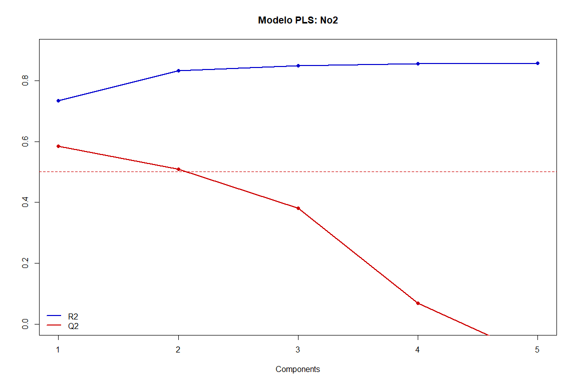
2.3 Partial Least Squares (PLS)

As previously observed, no2 has a positive correlation, although not very direct, with traffic. Next, we will study what factors can influence the formation of this chemical component using a technique called PLS., in English, Partial Least Squares.

This technique is a mix between multiple regression and PCA. Keep in mind that if there is multicollinearity, the regression may not be performed correctly and the desired results may not appear. However, the PLS previously uses the PCA to observe which variables are the most influential in the creation of the variables that are being studied and each of the components is orthogonal to the next one that most influences and so on. For that reason, thanks to the fact that the components are linearly independent from each other, the regression can be carried out without any problem.

In this case it can be seen that when applying the model, R2 is increasing, although not much, throughout the components that have been obtained. However, with Q2 the opposite happens, decreases from the second component.

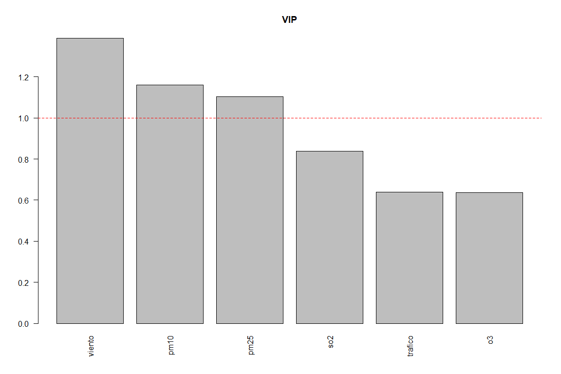
A technique that is widely used to obtain which variables have the most influence on the variable being predicted, VIP technique is used, that is to say, the influence of the variable Xi on the projection.

In this case, it can be seen how o3 and wind are the components that most influence the component of No2 because the VIP is greater than 1.

## traffic pm10 pm25 so2 o3 wind
## 0.6400664 1.1591929 1.1038898 0.8369390 0.6354506 1.3869931

Below is the graph of the weights in both space X and space Y to see how each of the regressors are distributed in addition to the variable being predicted, the no2.

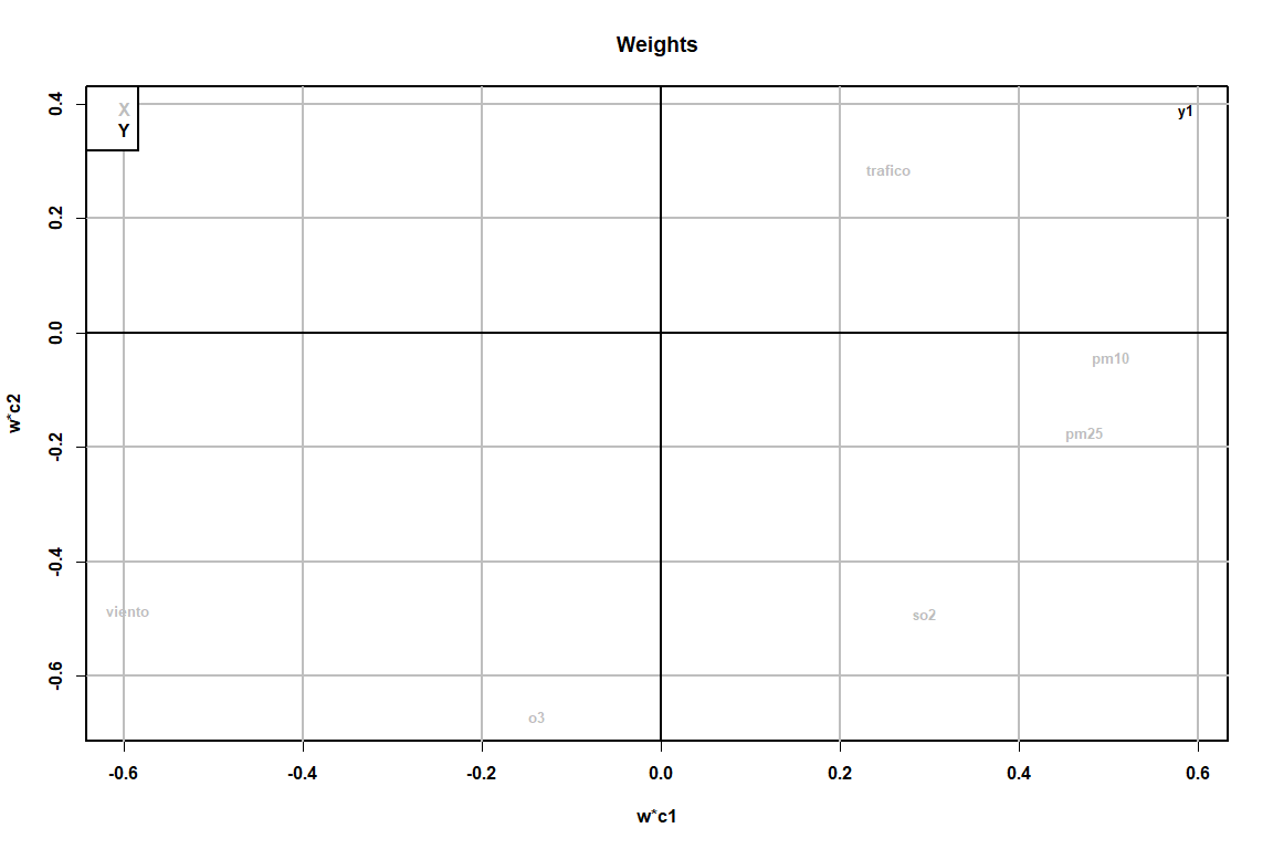
This chart is closely related to the VIP chart shown above. For example, observing the positions of the variable Y (No2) and the wind position you can tell that, the higher the wind, minor no2 will exist because the relationship is inverse.

Finally, a graph is attached that allows visualizing the internal relationship between the scores of space X (t) and the scores of the space Y (u).

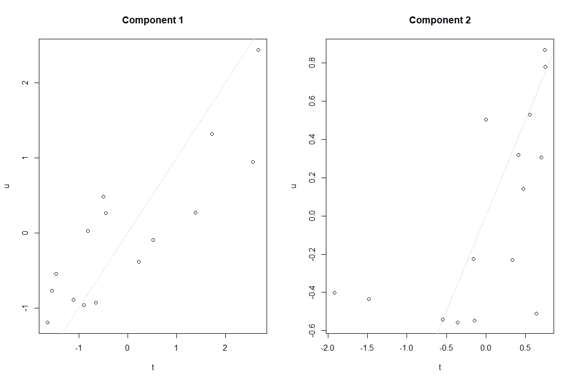
It can be seen that in the first component or dimension, the internal relationship between both scores is linear, Thus, no non-linear transformation would need to be applied to the model. However, in the second component, the relationship is not as clear as in the previous case.

3 Conclusions

Pollution and traffic 2020 (lockdown) compared to 2017

3.1 Traffic and pollution evolution comparing 2017 with 2020

For everything discussed above (pulled apart 1), it can be said that traffic and pollution in general has decreased markedly when comparing the period of 2017 with the of 2020 (with confinement). It must be emphasized that the study of the evolution of traffic and pollution has been carried out on a daily basis. This assumes that the data is aggregated and information is lost at the cost of generalizing. (get the average of the hours). Too, it should be noted that some pollutants such as O3 and SO2 have suffered little variation between years. Especially, el O3, has increased from 2017 a 2020, probably due to the mass use at present to disinfect objects.

3.2 Traffic and pollution relationship

For everything discussed above (pulled apart 2), It can be affirmed that traffic and pollution do not have a significant linear relationship since, in the models that have been obtained, the traffic parameter was never significant. It must be emphasized that, in the case of NO2 and PM10 pollutants, the p-value the parameters corresponding to the traffic are 0.39 and 0.38 respectively. Although they are far from 0.05 to be meaningful, are the highest p-values of all the models of pollutants, indicating that NO2 and PM10 pollutants have the highest linear relationship with traffic.

Too, it is necessary to emphasize the significance of the wind in different linear models, like the NO2, PM10 or O3, in all of them, with a higher level of confidence than 90%. This indicates that the wind has a linear relationship with these pollutants.

By last, mention the internal relationship between certain pollutants, like SO2.

3.3 General conclusions

Pollution and traffic 2020 (lockdown) compared to 2017

As seen previously, none of the models has been able to fit the data correctly since their fitted R squares are relatively low. Which is a possible indication that pollution depends on more variables than traffic or wind, how could the temperature be, the accumulated traffic and / or the type of vehicles that transit (trucks, motorcycles, etc…). For all this, it is not possible to obtain a model capable of estimating pollutants in a very approximate way, using only daily traffic and average wind speed. More explanatory variables are necessary.

It should also be noted that only linear relationships have been studied, so it is possible that there is another type of non-linear relationship between traffic and pollution.

AND, by last, must take into account, that traffic data comes from electromagnetic coil type sensors, these are the cheapest sensors that exist to measure traffic but also the most inaccurate, in addition to that the whole process of sending sensor data to the central server may fail, thus, Traffic data is not a very reliable source of information for modeling or analysis.

Bibliography:

Pollution and traffic 2020 (lockdown) compared to 2017

1 thought on “Pollution and traffic 2020 (lockdown) compared to 2017”

Michelle
25/06/2020 at 10:14 AM

I want to thank, this information adds value to us
as readers. I had read other blogs about it and I accept that this article explains the topic better.
I really appreciate the information.

Pollution and traffic 2020 (lockdown) compared to 2017

Introduction:

1. Analysis and evolution of traffic and pollution

-1.1 Average traffic during 15 days.

-1.2 Pollution levels of pollutants:

-1.2.1 NO2 (Nitrogen dioxide)

-1.2.2 PM10 (Suspended particles less than or equal to 10 microns per cubic meter)

-1.2.3 PM2.5 (Suspended particles less than or equal to 2.5 microns per cubic meter)

-1.2.4 SO2 (Sulfur dioxide)

-1.2.5 O3 (Ozone)

2 Traffic ratio – contamination

-2.1 Daily traffic correlation, wind and level of pollutants of the year 2020

2.2 Simple regression model

2.2.1 Input data

2.2.2 Model

2.2.2.1 NO2

2.2.2.2 PM10

2.2.2.3 PM2.5

2.2.2.4 SO2

2.2.2.5 O3

2.3 Partial Least Squares (PLS)

3 Conclusions

3.1 Traffic and pollution evolution comparing 2017 with 2020

3.2 Traffic and pollution relationship

3.3 General conclusions

Bibliography:

1 thought on “Pollution and traffic 2020 (lockdown) compared to 2017”

Leave a Comment Cancel Reply

Legal warning