
Application of statistical and predictive methods
(FAMD, Clustering y PLS-DA)
on cardiovascular data to obtain which variables cause heart problems.
Angel Langdon & Ignacio Cano
1. Description of the study and the database.
1.1 Study Description
In this study, an analysis of the relationship between some variables that indicate physical properties of the state of a person will be carried out. (detailed later) and whether or not you have a heart problem. Thus, the most significant variables will be obtained when determining if a person has a heart problem. Also, An attempt will be made to classify individuals according to their physical condition into two groups., if they have had a heart problem or not. The possibility of prediction using a PLS-DA model will also be studied..
1.2 Database Description
The database consists 14 variables and 303 observations. The variables we handle are common and easy to understand. Most of them deal with technical aspects of heart properties and levels of certain substances that are influential in determining the existence of heart disease.. Then, the 14 variables for greater clarity when performing the analysis, Furthermore, it is essential to know what the topic is about to carry out a good analysis.
- Age: The person's age in years
- Sex: The sex of the person (1 = macho, 0 = female)
- Pain_chest: The type of chest pain experienced
- Value 0 –> Angina typical
- Value 1 –> Atypical angina
- Value 2 –> Chest pain but not angina type
- Value 3 –> Asymptomatic pain
- (Angina = oppressive pain caused by insufficient blood supply <> to heart cells)
- p_sanguinea_mmHg: The person's resting blood pressure measured mm Hg upon hospital admission
- cholesterol: The person's cholesterol level measured in mg / dl
- hyperglycemia: Blood glucose level (free glucose in blood) fasting person (>120mg/dl, 1 = true ; 0 = false). If it is greater than 120mg / dl it is called hyperglycemia, and if the patient has hyperglycemia for a long time it contributes to the development of diabetes.
- electro_repost: A resting electrocardiogram of the person
- Value 0 –> normal
- Value 1 –> ST-T segment wave abnormality (associated with various heart problems depending on the type of abnormality)
- Value 2 –> Hypertrophy in the left datatricle (caused by high blood pressure, can cause a heart attack)
- beats_minute: The highest beats per minute recorded by the person
- angina_by_exercise: If angina has been caused by exercise (1 = yes; 0 = no)
- s_st: ST segment depression caused by physical exercise compared to ST segment depression when the patient is at rest is studied. The higher this value, the more likely you are to have a heart problem..
- pending_s_st: the slope of the ST segment at the exercise peak
- Value 1 –> Upward sloping
- Value 2 –> Flat earring
- Value 3 –> Negative slope
- It would be interesting to change these values to 1, 0 and -1 respectively to be a little bit more similar to what they represent.
- n_vasos_sanguineos: number of main blood vessels (0-3)
- default_type: It is a test made with a radioactive element (Thallium) injected into the blood stream of patients. This allows studying the blood flow both at rest and exercising:
- Value 3 –> Normal blood stream.
- Value 6 –> No blood flow is observed in the area, neither at rest nor exercising. (fixed defect)
- Value 7 –> No blood flow is observed in the area while exercising, but at rest. (reversible defect)
- problem_heart: Heart problem:
- Value 0 –> No
- Value 1 –> Yes
- Value 2 –> Yes, worst
- Value 3 –> Yes, much worse
- Value 4 –> Yes, worst possible
- It should be noted that the variable problem_heart It will serve as a reference to know if we can predict possible cases of heart problems from the values that individuals take in the rest of the variables.. Therefore, this variable will be taken as supplementary and will serve as a reference..
2. Initial exploratory analysis and pre-processing of data
2.1 Missing data
We check that there are no missing data, for this, a graph of missing data is shown according to variable
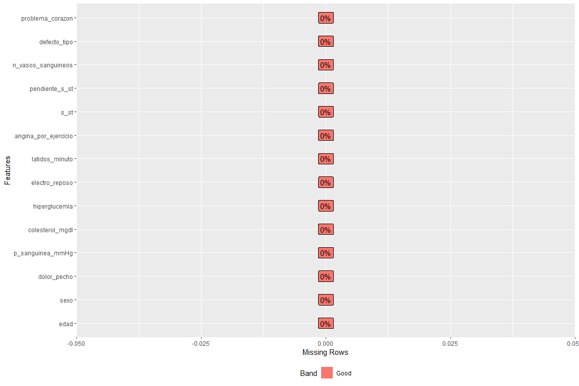
How can you see there is no empty field in any variable.
2.2 Variables and / or discarded records.
Doing a little research, this dataset in the blood vessel number column some observations take the value ?, which is wrong. (In the original dataset they represent NaNs). The same happens with the variable defect_type, who takes courage ?, it's bad. Therefore we will eliminate these observations
2.3 Recoding of variables
This step is performed in order to obtain more descriptive categories. In this way, categories that were previously “1” and “0” will become man and woman respectively.
2.4 Variable distribution
This step is carried out in order to observe what values the variables take and also to make sure that there are no erroneous values.
In the Annex 8.2: Variable distribution analysis is all explained
After studying the distribution of the variables, we observe none of them has wrong values, and therefore, we can continue with the analysis.
3. Analysis 1 FAMD(factominer)
FAMD (Mixed data factor analysis) is a principal component method dedicated to exploring data with continuous and categorical variables. Broadly speaking, it is a mixture of PCA and AFC.
Specific, continuous variables are scaled to unit variance and categorical variables are transformed to a disjunctive table and then scaled using AFC criteria. This makes both types of variables representative in the analysis.. That is to say, that one type of variables does not influence more than the other type of variables. In this case, corazón heart problem ’will be left as a supplementary variable, so that we can see if without their presence the individuals are divided into two groups as they would if said variable were present. If you want to find more information about FAMD you can do it at http://www.sthda.com/english/articles/31-principal-component-methods-in-r-practical-guide/115-famd-factor-analysis-of-mixed-data-in-r-essentials/ and also in https://rdrr.io/cran/FactoMineR/man/FAMD.html
3.1 goals
- Perform preprocessing of the data that is numerical and categorical to obtain its matrix of scores (with the most significant X main components) in order to be able to use it in Clustering (clustering does not support mixed data)
- Study the relationships between the variables of a person's physical state, leaving the heart problem variable as a supplement so that it does not influence the study and see if individuals, by themselves, they are divided into two groups (with a heart problem yes or no).
3.2 Application of the method and numerical and graphic results
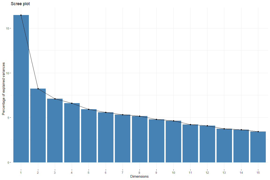
In the scree plot we can see how from the 6 dimension the contribution of the dimensions descends evenly. Thus, will be chosen 6 dimensions to represent our data. We also catch 6 dimensions since that way we get an explanation of 50% of variability. Now we are going to study the contribution of the variables to the first dimensions.
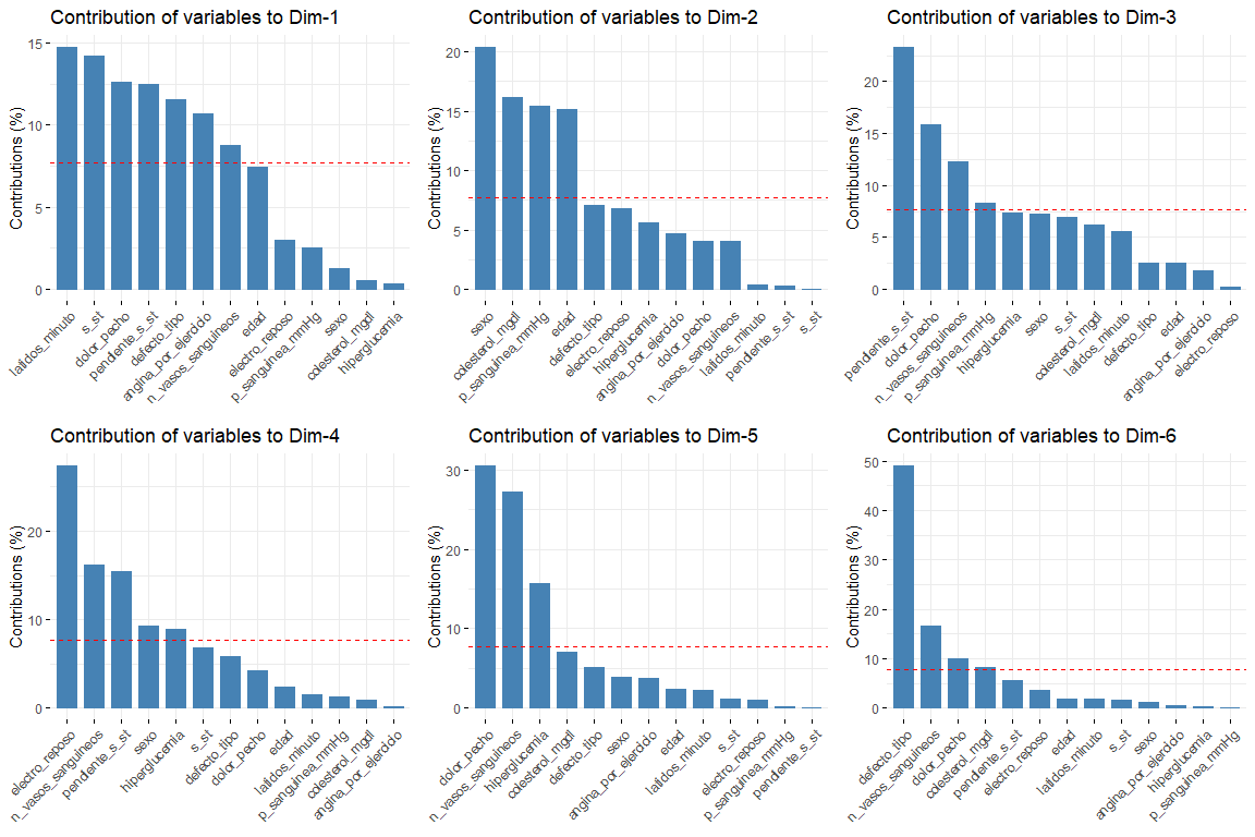
The most interesting results of the contributions are those of the first two dimensions (since they are the ones that explain the most variability). It should be noted that the first dimension is characterized by several variables (logical since it is the one that explains the most variability of all) these are default_type, pain_chest and st. In the second dimension, the number of variables that characterize this dimension is less than those of the first dimension, and these are sex, age, cholesterol_mgdl, p_sanguinea_mmHg. Once the first two dimensions are characterized, we will see the graph of variables drawn in the vector space of the first two dimensions, in order to observe the relationships between variables, and its characterization in each of the two dimensions in a more visual way.
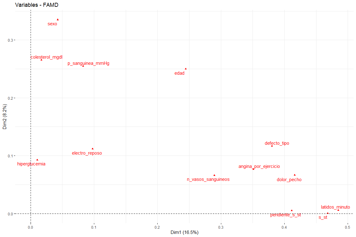
In this graph we can see represented the first two dimensions (the most important) and we have results that confirm those seen in the contribution graph. Variables such as latidos_minuto or s_st are the ones that contribute the most to the first dimension and the variables sex or age have a great contribution to the second dimension..
3.3 Discussion of results
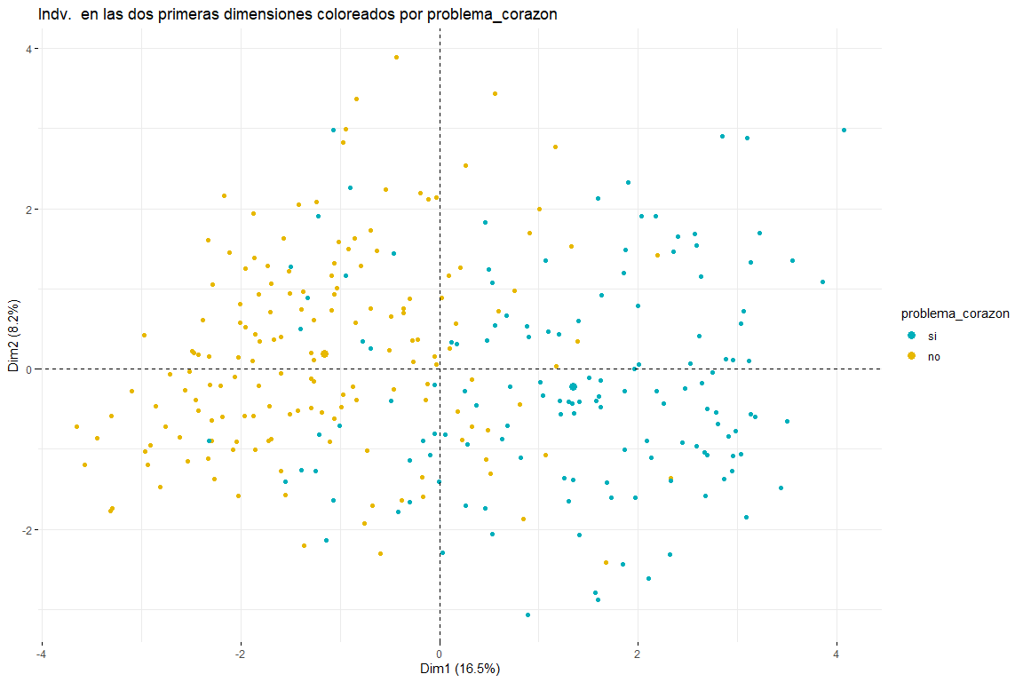
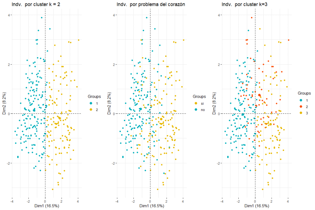
After seeing the graph of individuals colored by problema_corazon we can distinguish between two and three groups (for this, subsequent clustering analyzes would be necessary) both possible results make sense since two groups would imply that the values in certain variables (default_type, pain_chest, sex, age, cholesterol_mgdl, p_sanguinea_mmHg) imply the separation between cases of heart problems and those that do not. Three clusters could also make sense since seeing the graph we see how the values problem_heart = yes and problem_heart = no are separated, but we can also see how in the center the values of heart problem yes and heart problem no, therefore the presence of three clusters could also be possible. We can also affirm that the main direction of separation of the groups comes due to the first dimension., therefore the variables defect_type, pain_chest, s_st, default_type, p_sanguinea_mmHg would be those that would allow identifying those patients who have suffered a heart problem. It also appears that individuals who have had heart problems are not only displaced to the right but also down. This would imply that variables that contribute the most to the second dimension (sex, age, cholesterol_mgdl, p_sanguinea_mmHg) they would also have to do with identifying whether or not a patient has had a heart problem. These conclusions are expected to be confirmed with the subsequent clustering analysis from this FAMD analysis..
4. Hierarchical clustering
The HCPC (Hierarchical Clustering on Principal Components) is an algorithm that groups similar individuals into clusters but with a peculiarity. It is made to work with the results of a principal component method (PCA, MFA, FAMD…). For more information: http://www.sthda.com/english/articles/31-principal-component-methods-in-r-practical-guide/117-hcpc-hierarchical-clustering-on-principal-components-essentials/
4.1 objective
- Through the matrix of scores obtained in the FMAD, observe whether by performing hierarchical clustering with these individuals, two clusters are obtained that group the individuals into people with and without heart problems.. In case this doesn't happen, study the reason for the existence of the unexpected number of clusters.
4.2 Application of the method
To do the clustering we are going to use the coordinates of the individuals in the 6 dimensions that we have taken in the FAMD. The objective of the FAMD, as previously discussed, was to pre-process the data to be able to subsequently cluster. Nonetheless, We have obtained quite revealing results with the FAMD only and it is expected that with the clustering analysis these results will be confirmed..
For the calculation of the score matrix that will later be used in clustering, all the variables that indicate the physical state of the person will be used. It is emphasized that in the hierarchical clustering the variable problem_heart will NOT be included so that it has no effect when calculating the clusters. Since the objective is to calculate clusters through the variables of the physical state, to see if it's related to the heart problem.
4.2.1 We calculate the distances and the Hopkins statistic
Before applying any clustering algorithm it is important to ask yourself if there is any type of grouping for it, We perform the Hopkins statistic that indicates if there is a grouping in the data. We must remember that the library 'clustertend' returns 1-H with H being the Hopkins statistic.
$H
## [1] 0.2628502
In the case of heart data, the statistician has a value of 0.26 very far from 1, so, we can affirm that there is grouping in our data.
4.2.2 Optimal number of clusters
To be able to run the Hierarchical Clustering algorithm, we have to know the optimal number of clusters. For this we will run the following tests.
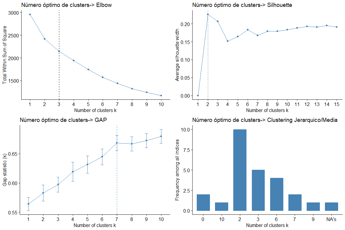
Looking at the graphs and tables we can see that for the different statistics and methods we obtain different values of clusters. The most frequent result is to consider 2 clusters, followed by 3 clusters. (the result 7 it also appears repeated but as it would not make sense to consider 7 groups we discard this conclusion)
Then, we make a cluster plot of 2 and 3 clusters respectively to see which one best fits our data. We use to obtain the kmeans data since when analyzing the data we can see that the data does not have very extreme values and therefore, no need for more robust methods like PAM, for example.
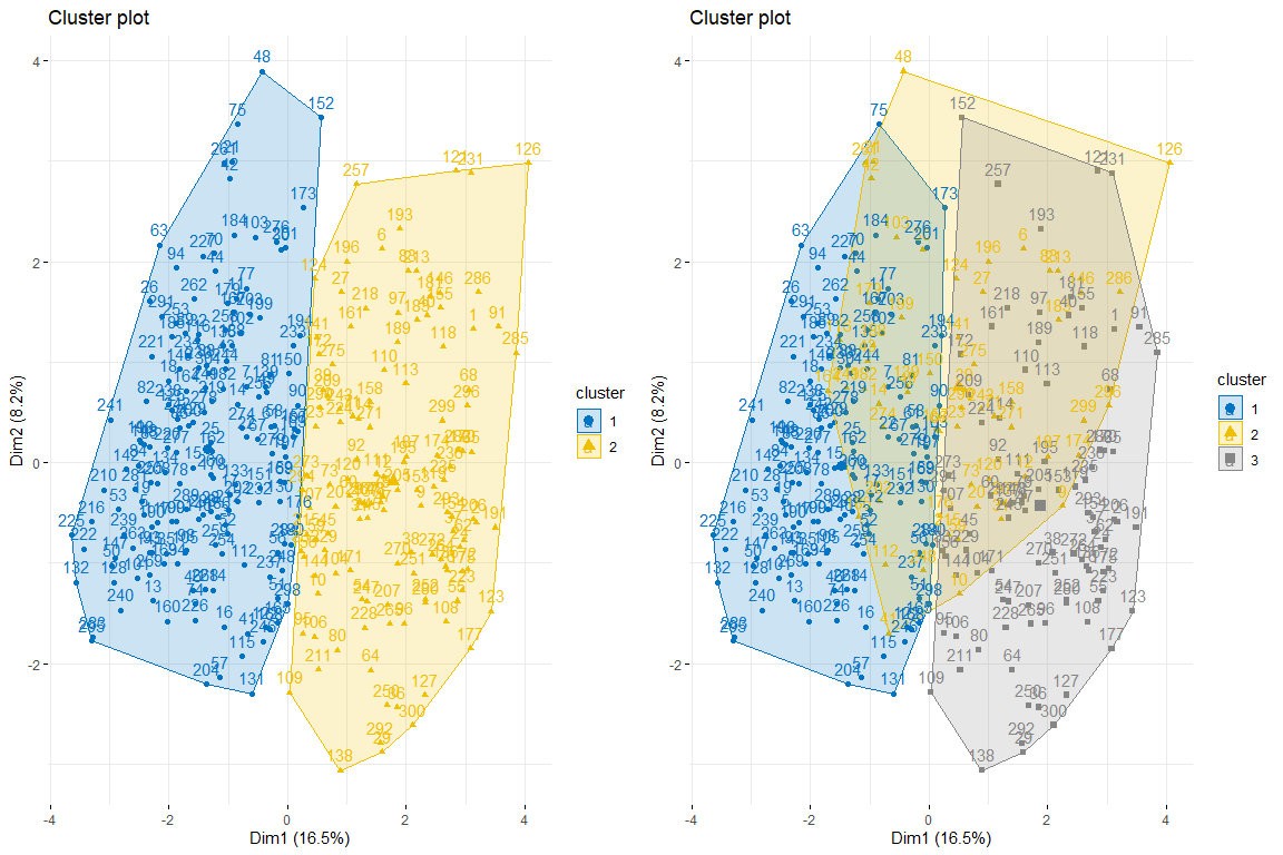
As we can observe 2 clusters seems to be the best option since it creates 2 pretty natural groups, that is to say, those individuals with heart problems and those who do not.
We will continue with the comparison between two and three clusters by coloring the individuals from the FAMD individuals plot..
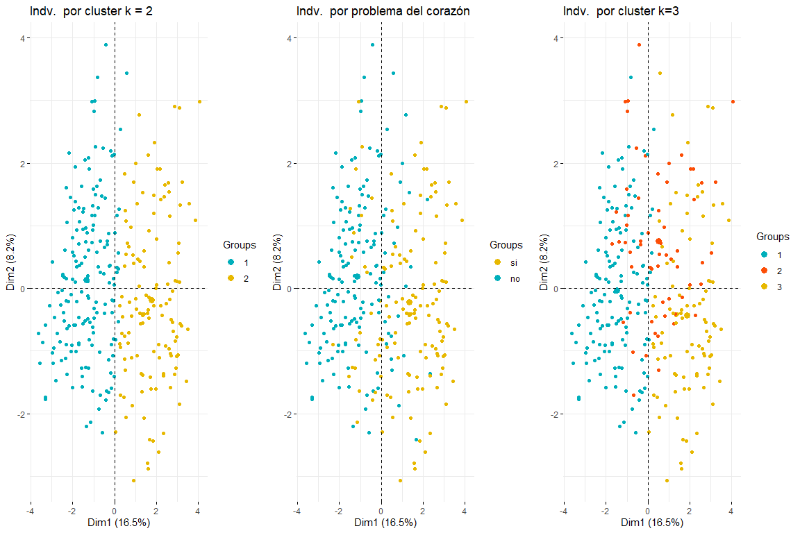
As can be seen in the three graphs of the individuals colored by cluster and by heart problem, it is appreciated that two clusters is the one that best adapts, and looks more like the chart of individuals colored by heart problem. After comparing these three groups of graphs we can conclude that using two clusters corresponds more to the distribution of the data according to problem_heart. For all this, two clusters will be chosen for hierarchical clustering.
4.3 Numerical and graphical results
Finally, the relationship between the variables and the two clusters and, Thus, their relationship with whether or not they have a heart problem. We will start with the relationship between the categories of qualitative variables and membership in one cluster or another. It is evident that those categories most related to a cluster are those with a higher v.test, while those whose value of v.test is very negative, less related will be with said cluster (and since we only have two clusters, probably these categories with a very negative v.test will be related to the other cluster.).
res.hcpc2$desc.var$category
## $`1`
## p.value v.test
## slope_s_st = positive 2.930295e-25 10.384064
## angina_por_exercise = angina_no_exercise 1.061236e-23 10.035774
## default_type = normal 2.733441e-22 9.709997
## n_vasos_sanguineos = 0 4.846452e-13 7.229537
## pain_chest = angina_atipica 4.782592e-11 6.577551
## pain_chest = pain_no_angina 1.569061e-07 5.244266
## sex = woman 4.235184e-05 4.094260
## electro_repost = normal 4.769950e-03 2.822173
## $`2`
## Cla / Mod Mod / Cla Global
## p.value v.test
## angina_por_exercise = angina_exercise 1.061236e-23 10.035774
## pendiente_s_st=plana 5.739929e-20 9.149120
## pain_chest = asymptomatic 8.164639e-19 8.857749
## defect_type = defect_reversible 2.547142e-15 7.911300
## sex = man 4.235184e-05 4.094260
## n_vasos_sanguineos = 2 4.952918e-05 4.057838
## n_vasos_sanguineos = 3 9.157912e-05 3.911883
## default_type = fixed_defect 1.073890e-04 3.873260
## n_vasos_sanguineos = 1 4.649990e-03 2.830331
## electro_reposto = hypertrophy_izq 2.225498e-02 2.285988
## electro_repost = abnormality_st 3.297443e-02 2.132394
## slope_s_st = negative 4.472770e-02 2.007206
Now we will see the relationship between the quantitative variables and the two clusters. The most representative variables are those with the highest v.test (in absolute value) and looking at the difference between ‘Mean in category’ and ‘Overall mean’ we can get an idea of what values individuals in a cluster take on these variables.
## $`1`
## v.test Mean in category Overall mean sd in category
## beats_minute 10.133353 161.3313609 149.597973 16.6608075
## p_sanguinea_mmHg -3.346967 128.6508876 131.648649 16.2372212
## age -6.575012 51.5147929 54.513514 8.9085469
## s_st -9.798909 0.4757396 1.051351 0.6908983
##
## $`2`
## v.test Mean in category Overall mean sd in category
## s_st 9.798909 1.817323 1.051351 1.222434
## age 6.575012 58.503937 54.513514 7.537699
## p_sanguinea_mmHg 3.346967 135.637795 131.648649 18.848618
## beats_minute -10.133353 133.984252 149.597973 20.744028
So that, you can see that the individuals that make up the first cluster are defined by having high values in beats_minute (with respect to the mean), low in age, p_sanguinea y s_st. We can also see how the individuals in the cluster 1, that is to say those cases that have not suffered a heart problem, they are women, whose chest pain is not atypical angina or angina and not caused by exercise. Also, your electro at rest is normal, its value after the test with Thalium is normal and its n_vasos_sanguíneos is 0.
On the other hand, the individuals in the second cluster are predominantly male, whose blood pressure is higher than average, whose beats per minute are less than the average and whose s_st is greater than the average. They also stand out for having a flat slope_st, some values of 1, 2 The 3 in n_vasos_sanguíneos, whose angina is caused by exercise, his pain is asymptomatic and his value after the Thalium test is reversible or fixed. Finally, its resting electro values are hypertrophy or abnormality_st.
4.4 Discussion of results
As you can see the variables that most characterize the clusters and consequently, also if a person has a heart problem or not, are those variables that made the greatest contribution to the first and second dimensions of the FAMD made previously. Also, we can see that the conclusions that have been obtained make sense; those who have suffered a heart problem (belonging to the cluster 2) have a very low maximum heart rate per minute, an advanced age, they are boys, higher than normal blood pressure, asymptomatic chest pain… all these are risk factors for cardiovascular problems.
5. Analysis 3: PLS-DA
The regression of partial least squares or Partial least squares regression (PLS regression) it is a statistical method that is related to the regression of principal components, instead of finding maximum variance hyperplanes between the response variable and the independent variables, a linear regression is found by projecting the prediction variables and the observable variables to a new space. Because both the X and Y data are projected into new spaces, the PLS family of models is known as the bilinear model factor. In our case, we will use partial least squares discriminant analysis (PLS-DA) which are a variant that is used when the Y is binary.
5.1 goals
There are two objectives when performing the PLS-DA:
The first is to compare the results obtained in the FAMD using the scores and loadings graphs and see if the same result can be interpreted. Also through the Observation Diagnostics graph we can observe the existence or not of extreme data.
The second objective is to evaluate the predictive capacity of the PLS-DA model with the data, which will be separated into training data and test data. This will serve to see if it is possible to predict new cases of heart problems with the available variables..
5.2 Application of the method
For the application of the method, a different pre-process of the ‘independent’ variables that will form our matrix X has been used, since the opls function needs all the columns of the matrix X to be of type ‘numeric’ (code available in Annex)
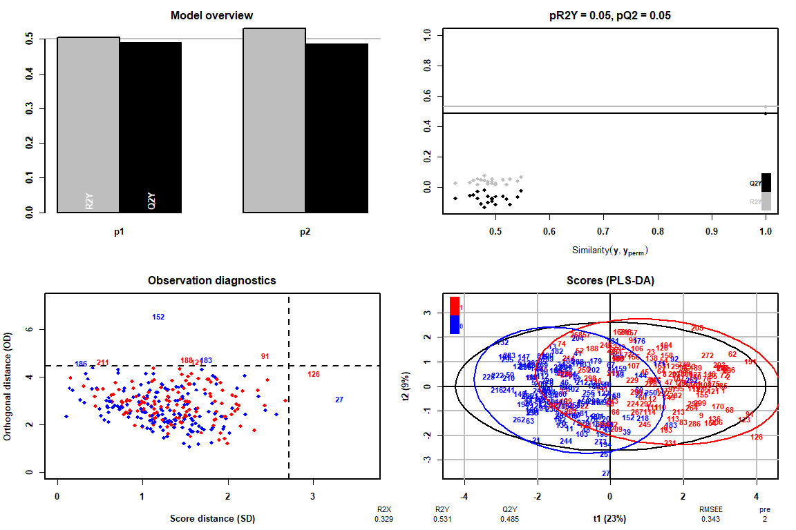
How it can be observed thanks to the Observation Diagnostics chart, there are no extreme values, therefore we can continue the analysis of the PLS-DA without having to delete any value.
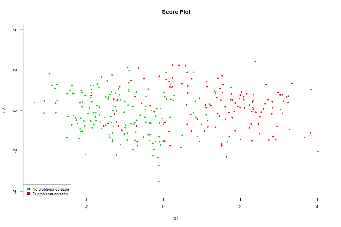
This graph is practically a copy of the one obtained in the FAMD, we see how clearly the points are separated into two groups (heart problem and not heart problem)
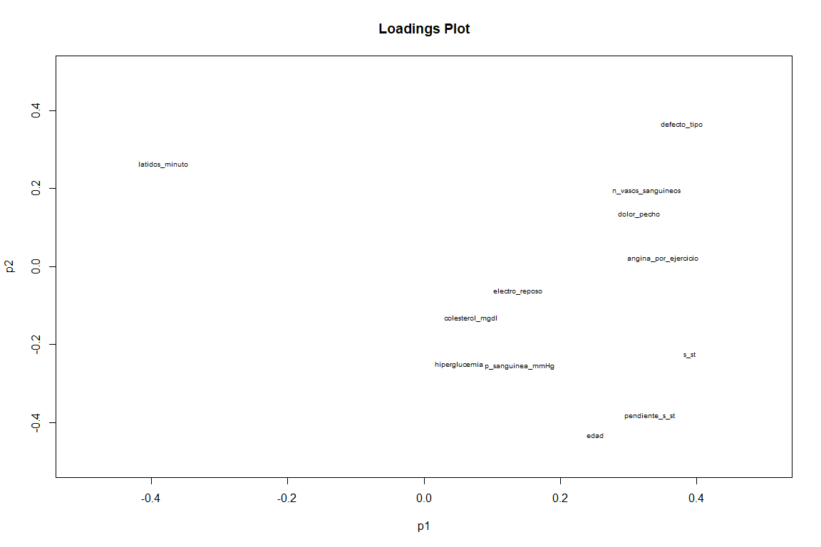
On the Loadings chart, if we see a somewhat different result from the FAMD loadings graph. We see as variables as slope_s_st, default_type and minute_beats (although this with negative value ) have a great contribution to the two components. While variables such as angina_por_exercicio and pain_chest contribute above all to the first component.
Now we turn to analyze the predictive capacity of the pls-da using training data and test data.
mypred = predict(myplsda)
confuTrain = table(trainData$problem_heart, mypred)
confusionMatrix(confuTrain)
## Confusion Matrix and Statistics
## mypred Accuracy : 0.8487
## 0 1 Kappa : 0.6946
## 0 113 15
## 1 21 89 Balanced Accuracy : 0.8495
How can we see the model predicting its own rows, It has an accuracy of 0.85, very good value that comes backed by a kappa 0.7, which indicates a good agreement of our data. (https://es.wikipedia.org/wiki/Coeficiente_kappa_de_Cohen)
Next thing is to try to predict data that the PLS-DA has never 'seen'
mypred = predict(myplsda, testdata[,–14])
confuTest = table(testdata$problem_heart, mypred)
confusionMatrix(confuTest)
## Confusion Matrix and Statistics
## mypred Accuracy : 0.8448
## 0 1
## 0 28 3 Kappa : 0.6859
## 1 6 21 Balanced Accuracy : 0.8493
The model has similar values (accuracy y kappa) for data you've never seen, with which it can be concluded that this model, predicts pretty well if a new case is going to have a heart problem or not with a probability of about 84% (Accuracy 0.84)
5.4 Discussion of results
You can see how PLS-DA is a very good method to predict new cases of heart problems in patients, However, It should be noted that the study consisted of some 300 patients approximately, so the number of individuals would have to be increased to see if this PLS-DA model really predicts with such certainty (84%) whether a patient will have a heart problem or not. On the other hand, Both the score matrix and the loadings matrix have been studied in two components. (the most significant) and the differences with the FAMD results have been studied.
6. Conclusions
6.1 Comparative methods used
In this work, three methods have been used: FAMD, Hierarchical clustering and PLS-DA.
Both the FAMD and the clustering have seen practically the same results (information found in the conclusions section of the respective method) this makes sense since the coordinates of the individuals in the first six main components have been used to perform the hierarchical clustering, therefore the FAMD has served us as data preprocessing (for clustering) and also as a first analysis of the relationships between variables and individuals in our database. In clustering we have confirmed those first observations we made about the existence of two groups and the variables that influence them.. The PLS-DA, although it has also been used to compare the results with those of the FAMD due to the possible similarity between the Scores and Loadings graphs., It has been mainly used to evaluate the predictive capacity of the model with our data.. Thus discovering the great predictive capacity of the model with an accuracy of 85% in data that I've never seen (test data).
6.2 Discussion on non-applied methods
The methods that have not been used in this work are: Association rules, discriminant analysis.
First, association rules are not used because we consider that it did not fit our database (our variables are not qualitative and the fact of transforming all the variables would have meant a significant loss of information). Instead, clustering and the possibility of actually being able to see the clusters into which our database was separated seemed to us a much more interesting option.
Regarding discriminant analysis, It is true that it would have been a very interesting option since precisely our intention from the first moment is to see the variables that are most related to having a heart problem or not., to then predict future cases or classify the individuals which we already had. However, the PLS or PLS-DA was mandatory to use and the FAMD and clustering analyzes had already been carried out, which are considered more relevant in this case than the discriminant analysis, therefore it has been decided to do without it.
By last, the choice between PLS and PLS-DA is obvious since the intention has always been to study the relationship between heart problem and the other variables, therefore the best option in this case is to choose PLS-DA, using as Y the heart problem and as X the rest of the variables to study the relationship between them and the ability to predict.
7 Other themes
7.1 Comments on articles read
The idea of removing both FAMD and hierarchical clustering (as well as using the score matrix for hierarchical clustering) ha surgido del libro ‘Practical Guide To Principal Component Methods in R (Kassambara)’ y del libro ‘Exploratory Multivariate Analysis by Example Using R (Chapman & Hall/CRC Computer Science & Data Analysis)By Francois Husson. We believe that it is a very powerful tool to combine both techniques (FAMD and clustering) since first, allows us to remove noise from our data, and second, using FAMD as preprocessed we can use ‘mixed data’ in clustering, which brings us a great benefit.
8. Annex:
8.1 Blibliography
- HCPC I
- FAMD I
- Pending ST segment information
- ‘Practical Guide To Principal Component Methods in R (Kassambara)’
- ‘Exploratory Multivariate Analysis by Example Using R (Chapman & Hall/CRC Computer Science & Data Analysis)By Francois Husson
- FactoMineR Documentation
- Changes in the heart and blood vessels due to aging
- Maximum beats per minute
- Risk factors for cardiovascular problems
- Data used
8.2 Variable distribution analysis
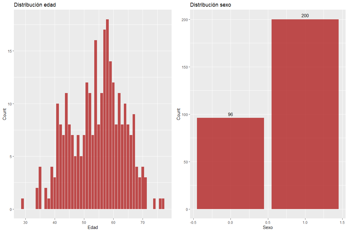
The age variable does not take extreme values and the sex variable does not contain erroneous values.
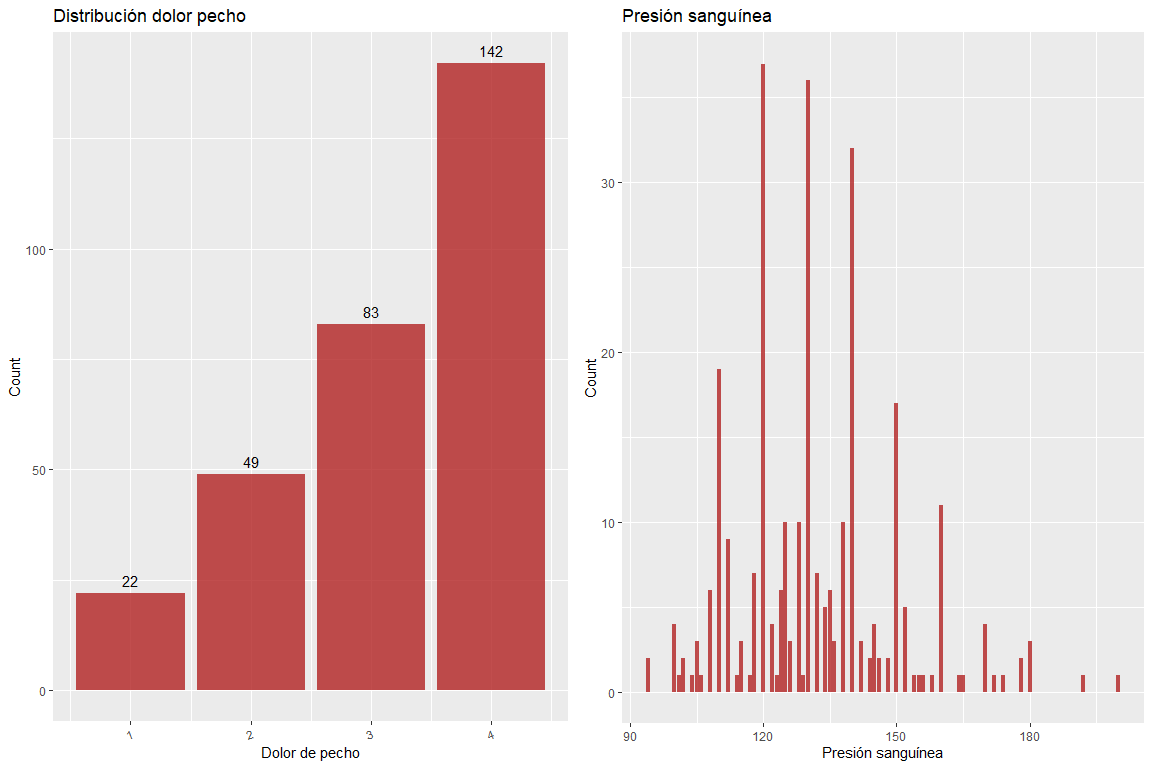
Variable chest pain does not contain wrong values, just as neither does the variable blood pressure.
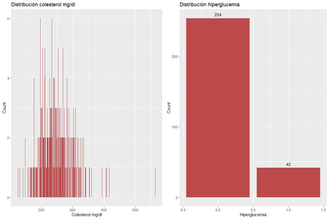
The two variables Cholesterol mg / dl and hyperglycemia do not take wrong values.
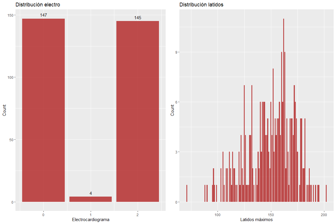
The two variables results of the electrocardiogram and maximum beats per minute do not take wrong values.. However, it must be emphasized that there are somewhat high values for the age of the patients. (according to Haskell's formula & Fox, The use of which is widely used to delimit the maximum pulsations according to age).
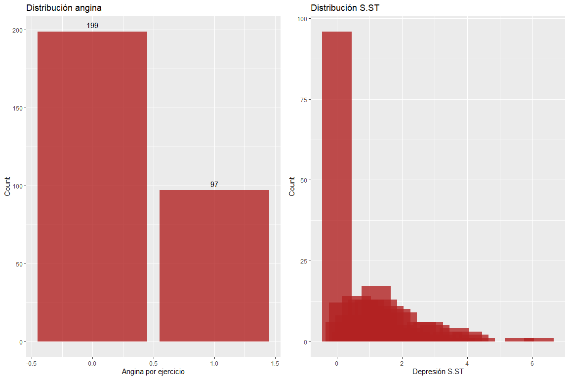
The two variables exercise angina and depression of the ST segment do not have erroneous values.. But it must be emphasized that there are observations with a very high ST segment depression value.
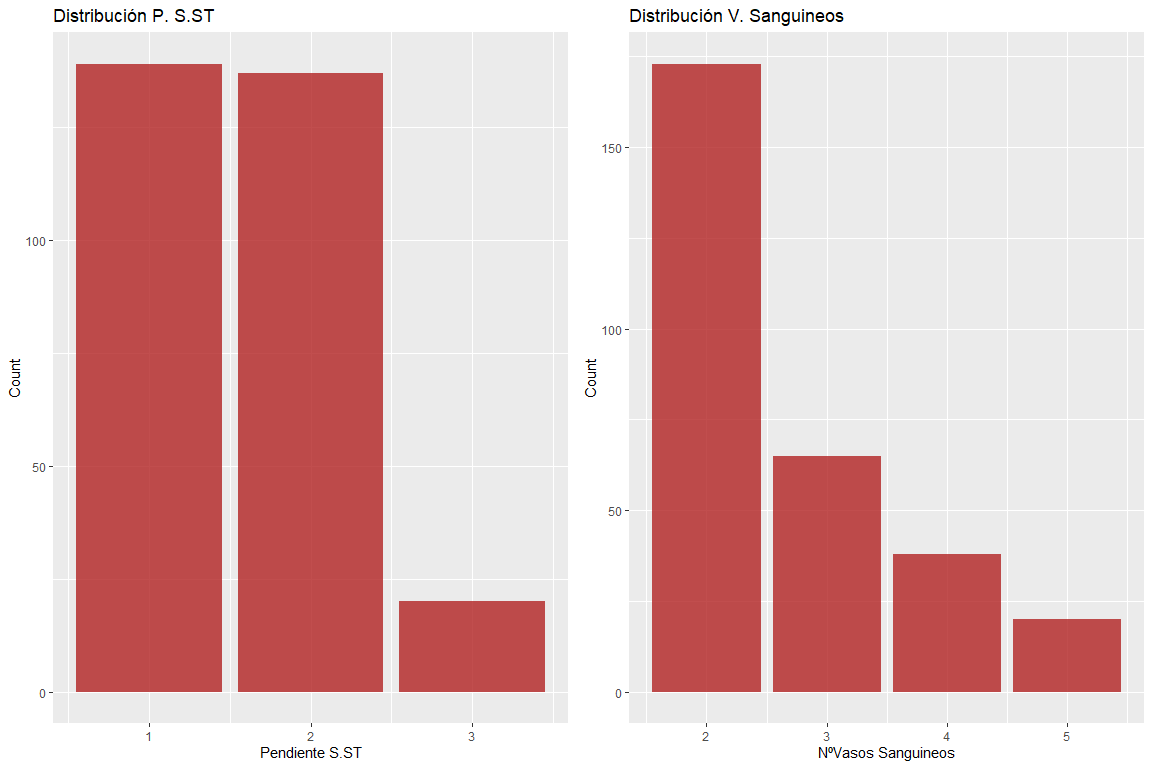
The two variables pending ST segment and number of blood vessels do not have erroneous values.
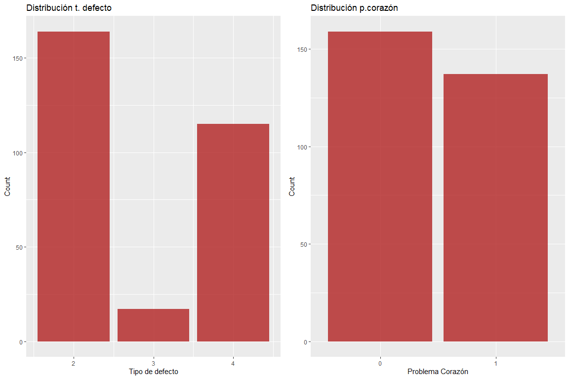
The two variables type of defect and heart problem do not have erroneous values.